Contents
tVAE
from atomai import stat as atomstat
import atomai as aoi

import numpy as np
import pyroved as pv
import gdown

import torch
import random
tt = torch.tensor

torch.manual_seed(0)
# torch.cuda.manual_seed_all(0)
# torch.backends.cudnn.deterministic=True
np.random.seed(0)
random.seed(0)

import os
import wget
from sklearn.preprocessing import StandardScaler
import h5py
import matplotlib.pyplot as plt
from sklearn.mixture import GaussianMixture
from sklearn.decomposition import PCA
from skimage import feature
import skimage
from scipy.ndimage import zoom
from matplotlib.patches import Rectangle
import seaborn as sns
import ipywidgets as widgets
from ipywidgets import interact

import ipywidgets
import pickle
from ipywidgets import interact, Layout
from IPython.display import display, HTML
/tmp/ipykernel_266104/4005104371.py:36: DeprecationWarning: Importing display from IPython.core.display is deprecated since IPython 7.14, please import from IPython.display
  from IPython.core.display import display, HTML
Load imaging data
# ! gdown --fuzzy --id 1AHlk5xxXiuiTtYNr8fk0YQ8Uxjbf8bfTid="1AHlk5xxXiuiTtYNr8fk0YQ8Uxjbf8bfT"
if not os.path.exists("data/images_data.pkl"):
gdown.download(id=id,fuzzy=True,output="data/")# Load the lists from the pickle file
images_data = "data/images_data.pkl"
with open(images_data, "rb") as f:
selected_images, ground_truth_px, ground_truth_py = pickle.load(f)
# Confirm successful loading by checking the lengths of the lists
print(len(selected_images), len(ground_truth_px), len(ground_truth_py))5 5 5
# min-max normalization:
def norm2d(img: np.ndarray) -> np.ndarray:
    return (img - np.min(img)) / (np.max(img) - np.min(img))
image = selected_images[0]
img = norm2d(image)def custom_extract_subimages(imgdata, coordinates, w_prime):
# Stage 1: Extract subimages with a fixed size (64x64)
large_window_size = (64, 64)
half_height_large = large_window_size[0] // 2
half_width_large = large_window_size[1] // 2
subimages_largest = []
coms_largest = []
for coord in coordinates:
cx = int(np.around(coord[0]))
cy = int(np.around(coord[1]))
top = max(cx - half_height_large, 0)
bottom = min(cx + half_height_large, imgdata.shape[0])
left = max(cy - half_width_large, 0)
right = min(cy + half_width_large, imgdata.shape[1])
subimage = imgdata[top:bottom, left:right]
if subimage.shape[0] == large_window_size[0] and subimage.shape[1] == large_window_size[1]:
subimages_largest.append(subimage)
coms_largest.append(coord)
# Stage 2: Use these centers to extract subimages of window size `w1`
half_height = w_prime[0] // 2
half_width = w_prime[1] // 2
subimages_target = []
coms_target = []
for coord in coms_largest:
cx = int(np.around(coord[0]))
cy = int(np.around(coord[1]))
top = max(cx - half_height, 0)
bottom = min(cx + half_height, imgdata.shape[0])
left = max(cy - half_width, 0)
right = min(cy + half_width, imgdata.shape[1])
subimage = imgdata[top:bottom, left:right]
if subimage.shape[0] == w_prime[0] and subimage.shape[1] == w_prime[1]:
subimages_target.append(subimage)
coms_target.append(coord)
return np.array(subimages_target), np.array(coms_target)def build_descriptor(window_size, min_sigma, max_sigma, threshold, overlap):
processed_img = img
all_atoms = skimage.feature.blob_log(processed_img, min_sigma, max_sigma, 30, threshold, overlap)
coordinates = all_atoms[:, : -1]
# Extract subimages
subimages_target, coms_target = custom_extract_subimages(processed_img, coordinates, window_size)
# Build descriptors
descriptors = [subimage.flatten() for subimage in subimages_target]
descriptors = np.array(descriptors)
return descriptors, coms_target, all_atoms, coordinates, subimages_targetNow we know the optimum hyperparameters
window_size = (40,40)
min_sigma = 1
max_sigma = 5
threshold = 0.025
overlap = 0.0
descriptors, coms_target, all_atoms, coordinates, subimages_target = build_descriptor(window_size, min_sigma, max_sigma, threshold, overlap)
print(descriptors.shape)
print(coms_target.shape)
print(all_atoms.shape)
print(coordinates.shape)
print(subimages_target.shape)(10917, 1600)
(10917, 2)
(11813, 3)
(11813, 2)
(10917, 40, 40)
#normalize imagestack
subimages_target = subimages_target/subimages_target.max()
subimages_target = np.expand_dims(subimages_target, axis=-1)
train_data = torch.tensor(subimages_target[:,:,:,0]).float()
train_loader = pv.utils.init_dataloader(train_data.unsqueeze(1), batch_size=48, seed=0)
# in_dim = (window_size[0],window_size[1])
# # Initialize vanilla VAE
# tvae = pv.models.iVAE(in_dim, latent_dim=2, # Number of latent dimensions other than the invariancies
# hidden_dim_e = [512, 512],
# hidden_dim_d = [512, 512], # corresponds to the number of neurons in the hidden layers of the decoder
# invariances=["t"], seed=0)
# # Initialize SVI trainer
# trainer = pv.trainers.SVItrainer(tvae)
# # Train for n epochs:
# for e in range(10):
# trainer.step(train_loader)
# trainer.print_statistics()
# tvae.save_weights('tvae_model')
# print("Model saved successfully.")Load the pretrained model
# ! gdown --fuzzy --id 1x0SS4vvn1f62n3ZiRLUuonUVc8IKCaNPin_dim = (window_size[0],window_size[1])
# Reinitialize the model before loading weights
tvae_model = pv.models.iVAE(in_dim, latent_dim=2, # Number of latent dimensions other than the invariancies
hidden_dim_e = [512, 512],
hidden_dim_d = [512, 512], # corresponds to the number of neurons in the hidden layers of the decoder
invariances=["t"], seed=0)
# Load the saved model weights
tvae_model.load_weights('data/tvae_model.pt')
print("Model loaded successfully.")Model loaded successfully.
Varitional Auto Encoder manifold representation
rvae_laten_img = tvae_model.manifold2d(d=10, draw_grid = True, origin = 'lower')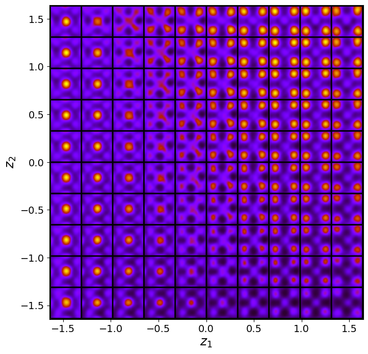
The latent representation of the system is visualized as a grid over the two latent variables and . Each grid cell corresponds to a unique combination of values for and , which are decoded to produce corresponding reconstructions in the data space. The smooth and structured transition across the grid indicates that the model has learned a meaningful and continuous mapping between the latent variables and the data space. Variations in the grid reflect changes in the underlying physical structure, such as column type, domain orientation, or material properties.
tvae_z_mean, rvae_z_sd = tvae_model.encode(train_data)
print('no. of defects', tvae_z_mean.shape)

z1 = tvae_z_mean[:, -2]
z2 = tvae_z_mean[:, -1]
tx = tvae_z_mean[:, -4]
ty = tvae_z_mean[:, -3]
no. of defects torch.Size([10917, 4])
def generate_latent_manifold(n=10, decoder=None, target_size=(28, 28)):
    """
    Generate a general latent manifold grid over the entire latent space.
    """
    # Define grid bounds across latent space
    grid_x = np.linspace(min(z1), max(z1), n)
    grid_y = np.linspace(min(z2), max(z2), n)

    # Dynamically infer output shape
    sample_input = torch.tensor([[grid_x[0], grid_y[0]]], dtype=torch.float32)
    with torch.no_grad():
        X_decoded = decoder(sample_input)
    decoded_shape = X_decoded.shape[-2:] if len(X_decoded.shape) > 2 else (X_decoded.shape[-1], X_decoded.shape[-1])

    height, width = target_size
    manifold = np.zeros((height * n, width * n))

    # Generate manifold
    for i, yi in enumerate(grid_x):
        for j, xi in enumerate(grid_y):
            Z_sample = torch.tensor([[xi, yi]], dtype=torch.float32)
            with torch.no_grad():
                X_decoded = decoder(Z_sample).reshape(decoded_shape)
            resized_image = zoom(X_decoded, zoom=(height / X_decoded.shape[-2], width / X_decoded.shape[-1]))
            manifold[i * height: (i + 1) * height, j * width: (j + 1) * width] = resized_image
    return manifold
# Apply styling for dropdowns
display(HTML("""
<style>
.widget-label { font-size: 16px; font-weight: bold; }
select { font-size: 16px; font-weight: bold; }
</style>
"""))
# Define dropdown styling
dropdown_style = {'description_width': 'initial'}
dropdown_layout = Layout(width='250px')
# Define available options for Panel B
options = ["z1", "z2", "tx", "ty"]
# Define a dictionary for mapping options to variables
variable_map = {
"z1": (z1, r"$z_1$", "plasma", "cyan"),
"z2": (z2, r"$z_2$", "plasma", "magenta"),
"tx": (tx, r"$t_x$", "plasma", "green"),
"ty": (ty, r"$t_y$", "plasma", "orange"),
}
def interactive_plot(variable_x, variable_y):
"""Creates a figure with fixed manifold (A) and interactive scatter plot (B)."""
fig, axes = plt.subplots(1, 2, figsize=(12, 6))
# **Panel A (Left) - Fixed Manifold**
manifold = generate_latent_manifold(n=10, decoder=tvae_model.decode, target_size=(28, 28))
axes[0].imshow(manifold, cmap="gnuplot2", origin="upper")
axes[0].set_xlabel(r"$z_1$", fontsize=16, fontweight="bold")
axes[0].set_ylabel(r"$z_2$", fontsize=16, fontweight="bold")
axes[0].set_xticks([])
axes[0].set_yticks([])
axes[0].text(-0.07, 1, 'a)', transform=axes[0].transAxes, fontsize=16, fontweight='bold', va='top', ha='right')
# **Panel B (Right) - Interactive Scatter Plot**
var_x, label_x, cmap_x, color_x = variable_map[variable_x]
var_y, label_y, cmap_y, color_y = variable_map[variable_y]
# Scatter plot
sns.scatterplot(x=var_x, y=var_y, ax=axes[1], color="blue", alpha=0.4, edgecolor="k", s=10)
# **Fix: Use PyTorch's Variance Instead of NumPy**
if torch.var(var_x) > 0 and torch.var(var_y) > 0:
sns.kdeplot(x=var_x.detach().cpu(), y=var_y.detach().cpu(), ax=axes[1], cmap="plasma", levels=50, thresh=0.05, alpha=0.4, fill=False, warn_singular=False)
axes[1].set_xlabel(label_x, fontsize=16, fontweight="bold")
axes[1].set_ylabel(label_y, fontsize=16, fontweight="bold")
axes[1].text(-0.07, 1, 'b)', transform=axes[1].transAxes, fontsize=16, fontweight='bold', va='top', ha='right')
plt.tight_layout()
plt.show()Loading...
# Create interactive dropdown widgets
interact(interactive_plot,
         variable_x=widgets.Dropdown(options=options, description="X-Axis", style=dropdown_style, layout=dropdown_layout),
         variable_y=widgets.Dropdown(options=options, description="Y-Axis", style=dropdown_style, layout=dropdown_layout)
        );
Loading...
<function __main__.interactive_plot(variable_x, variable_y)># Apply styling for dropdowns
display(HTML("""
<style>
.widget-label { font-size: 16px; font-weight: bold; }
select { font-size: 16px; font-weight: bold; }
</style>
"""))
# Define dropdown styling
dropdown_style = {'description_width': 'initial'}
dropdown_layout = Layout(width='250px')
# Define available options
options = ["z1", "z2", "tx", "ty", "Ground Truth Px", "Ground Truth Py"]
# Define variables
Px = ground_truth_px[0]
Py = ground_truth_py[0]
# Define a dictionary for mapping options to data and plot type
plot_data = {
"z1": {"data": z1, "type": "scatter", "title": "Latent Variable z1"},
"z2": {"data": z2, "type": "scatter", "title": "Latent Variable z2"},
"tx": {"data": tx, "type": "scatter", "title": "Translation X (tx)"},
"ty": {"data": ty, "type": "scatter", "title": "Translation Y (ty)"},
"Ground Truth Px": {"data": Px, "type": "image", "title": "Ground Truth Px"},
"Ground Truth Py": {"data": Py, "type": "image", "title": "Ground Truth Py"},
}
def plot_variable(ax, variable, subplot_label):
"""Plots the selected variable in the given axis."""
data = plot_data[variable]["data"]
plot_type = plot_data[variable]["type"]
if plot_type == "scatter":
ax.scatter(coms_target[:, 1], coms_target[:, 0], c=data, s=14, cmap='jet', marker="o")
elif plot_type == "image":
ax.imshow(data, cmap='jet', origin='lower')
ax.axis("off")
ax.text(-0.05, 1, subplot_label, transform=ax.transAxes, fontsize=16, fontweight='bold', va='top', ha='right')
def plot_two_variables(variable1, variable2):
"""Creates a 1-row, 2-column figure and plots two selected variables."""
fig, axes = plt.subplots(1, 2, figsize=(12, 6))
plot_variable(axes[0], variable1, 'a)')
plot_variable(axes[1], variable2, 'b)')
plt.tight_layout()
plt.show()
Loading...
# Create interactive dropdown widgets
interact(plot_two_variables,
         variable1=widgets.Dropdown(options=options, description="Variable 1", style=dropdown_style, layout=dropdown_layout),
         variable2=widgets.Dropdown(options=options, description="Variable 2", style=dropdown_style, layout=dropdown_layout)
        );
Loading...
<function __main__.plot_two_variables(variable1, variable2)>
