main
# ! pip install wget# ! pip install -q git+https://github.com/pycroscopy/atomai# ! pip install -q kornia atomai git+https://github.com/ziatdinovmax/pyroVED@main# ! pip install seabornImport libraries
#from atomai import utils
from atomai import stat as atomstat
import atomai as aoi
#from atomai import utils
# from atomai import stat as atomstat
# import atomai as aoi
import numpy as np
import pyroved as pv
import torch
import random
tt = torch.tensor
# Setting seeds to reproduce the results
torch.manual_seed(0)
torch.cuda.manual_seed_all(0)
torch.backends.cudnn.deterministic=True
np.random.seed(0)
random.seed(0)import os
import wget
from sklearn.preprocessing import StandardScaler
import h5py
import matplotlib.pyplot as plt
from sklearn.mixture import GaussianMixture
from sklearn.decomposition import PCA
from skimage import feature
import skimage
from scipy.ndimage import zoom
from matplotlib.patches import Rectangle
# import seaborn as sns
import ipywidgets as widgets
from ipywidgets import interact
import ipywidgetsimport seaborn as snsUpload Dataset
The dataset we have plan to work on represents unit cell (UC) information, and crystallographic properties of Sm-doped BiFeO₃ . Here’s an explanation of each parameter in this context:
I1, I2, I3, I4, I5: These correspond to intensity measurements at specific points or regions in the unit cell.
NCOM (Number of Centers of Mass): Indicates the number of calculated or observed centers of mass within the unit cell. This parameter could be used to understand atomic or molecular arrangement in the unit cell.
PCOM (Primary Center of Mass): Refers to the primary center of mass for the unit cell, potentially indicating the most significant mass concentration point. This can help in analyzing symmetry or balancing structural information.
Pxy: Pxy would specifically quantify the in-plane polarization vector within the x and y dimensions. The values in Pxy are essential for understanding how the electric dipole moments are distributed within the unit cell and whether there are tendencies for domains to form or align under external fields.
Vol (Volume): Refers to the volume of the unit cell, which is essential for calculations related to density and lattice spacing. Changes in volume can signal phase transitions or structural changes under different conditions.
a, b: These are lattice parameters along two main crystallographic axes. In crystallography, the lattice constants define the periodicity and distances between atoms in each direction.
ab, adelta, bdelta:
ab: Likely the in-plane lattice parameter, which might be averaged or specific to the ‘a’ and ‘b’ directions combined. adelta and bdelta: Represent the deviations or variations in the lattice parameters a and b, which can indicate strain or defects within the crystal structure. alpha: Typically represents an angle in crystallography (e.g., between lattice vectors), providing information about the unit cell’s geometry (e.g., whether it’s orthorhombic, monoclinic, etc.).
atmindex (Atom Index): An identifier for different atoms within the unit cell, essential for linking positional data with specific atoms.
index: Possibly a general identifier or label for the unit cell instance within the dataset, useful for tracking or referencing each cell.
meanuca and meanucb: Likely represent the mean values of the lattice parameters ‘a’ and ‘b’ across the dataset or a subset of unit cells, providing an average view of these dimensions.
nbrUC (Number of Unit Cells): Indicates the number of unit cells considered in this particular dataset or measurement set. This provides context for scale and sample size.
xy_COM (xy Center of Mass): X and Y coordinates of the center of mass for the unit cell, helpful for assessing symmetry and spatial positioning within the plane.
xy_atms (xy Atom Positions): The X and Y coordinates of atoms within the unit cell, specifying their positions relative to the cell origin, which is essential for visualizing and analyzing the atomic arrangement.
Each Sm_0_0_HAADF.h5 contains the Scanning Transmission Electron Microscopy (STEM) image for Sm-substituted BiFeO₃ (SmBFO) for different compositions.
# model_files = ['Sm_0_0_HAADF.h5','Sm_0_1_HAADF.h5','Sm_0_2_HAADF.h5',
#                'Sm_0_0_UCParameterization.h5','Sm_0_1_UCParameterization.h5','Sm_0_2_UCParameterization.h5',
#                'Sm_7_0_HAADF.h5','Sm_7_1_HAADF.h5', 'Sm_7_2_HAADF.h5', 'Sm_7_3_HAADF.h5', 'Sm_7_4_HAADF.h5',
#                'Sm_7_0_UCParameterization.h5','Sm_7_1_UCParameterization.h5','Sm_7_2_UCParameterization.h5','Sm_7_3_UCParameterization.h5','Sm_7_4_UCParameterization.h5',
#                'SM_10_0_HAADF.h5','Sm_10_1_HAADF.h5',
#                'Sm_10_0_UCParameterization.h5','Sm_10_1_UCParameterization.h5',
#                'Sm_13_0_HAADF.h5','Sm_13_1_HAADF.h5',
#                'Sm_13_0_UCParameterization.h5','Sm_13_1_UCParameterization.h5',
#                'Sm_20_0_HAADF.h5','Sm_20_1_HAADF.h5',
#                'Sm_20_0_UCParameterization.h5','Sm_20_1_UCParameterization.h5']

# for model_file in model_files:
#   print(model_file)
#   wget.download("https://zenodo.org/record/4555979/files/"+model_file+"?download=1", out=model_file)
model_files = ['Sm_0_1_HAADF.h5',
'Sm_0_1_UCParameterization.h5',
'Sm_7_0_HAADF.h5',
'Sm_7_0_UCParameterization.h5',
'SM_10_0_HAADF.h5',
'Sm_10_0_UCParameterization.h5',
'Sm_13_0_HAADF.h5',
'Sm_13_0_UCParameterization.h5',
'Sm_20_1_HAADF.h5',
'Sm_20_1_UCParameterization.h5']
for model_file in model_files:
print(model_file)
wget.download("https://zenodo.org/record/4555979/files/"+model_file+"?download=1", out=model_file)Sm_0_1_HAADF.h5
Sm_0_1_UCParameterization.h5
Sm_7_0_HAADF.h5
Sm_7_0_UCParameterization.h5
SM_10_0_HAADF.h5
Sm_10_0_UCParameterization.h5
Sm_13_0_HAADF.h5
Sm_13_0_UCParameterization.h5
Sm_20_1_HAADF.h5
Sm_20_1_UCParameterization.h5
#list files
filedir = '/Users/kbarakat/Library/CloudStorage/OneDrive-UniversityofTennessee/Documents/ferro_VAE/notebooks'
[f for f in os.listdir(filedir)]
['.DS_Store',
'Ferro_VAE_SmBFO.ipynb',
'Sm_0_1_UCParameterization.h5',
'Sm_13_0_HAADF.h5',
'Sm_7_0_UCParameterization.h5',
'Sm_7_0_HAADF.h5',
'SM_10_0_HAADF.h5',
'Sm_13_0_UCParameterization.h5',
'Sm_10_0_UCParameterization.h5',
'.ipynb_checkpoints',
'example_notebook.ipynb',
'Sm_20_1_HAADF.h5',
'Sm_20_1_UCParameterization.h5',
'Sm_0_1_HAADF.h5']filedir = '/Users/kbarakat/Library/CloudStorage/OneDrive-UniversityofTennessee/Documents/ferro_VAE/notebooks'
#image files
composition_tags = [0,7,10,13,20] #Sm composition %
img_filename = ['Sm_0_1_HAADF.h5',
'Sm_7_0_HAADF.h5',
'SM_10_0_HAADF.h5',
'Sm_13_0_HAADF.h5',
'Sm_20_1_HAADF.h5']
imnum = len(img_filename)
#paramterization files
UCparam_filename = ['Sm_0_1_UCParameterization.h5',
'Sm_7_0_UCParameterization.h5',
'Sm_10_0_UCParameterization.h5',
'Sm_13_0_UCParameterization.h5',
'Sm_20_1_UCParameterization.h5']
#load parameter files
UCparam = []
for x in UCparam_filename:
print('loading parameterization file: ', os.path.join(filedir, x))
temp = h5py.File(os.path.join(filedir, x), 'r')
UCparam.append(temp)
#load images
imgdata = []
for x in img_filename:
print('loading image file: ', os.path.join(filedir, x))
temp = h5py.File(os.path.join(filedir, x), 'r')['MainImage']
imgdata.append(temp)
print('UC parameterization:', [k for k in UCparam[0].keys()])loading parameterization file: /Users/kbarakat/Library/CloudStorage/OneDrive-UniversityofTennessee/Documents/ferro_VAE/notebooks/Sm_0_1_UCParameterization.h5
loading parameterization file: /Users/kbarakat/Library/CloudStorage/OneDrive-UniversityofTennessee/Documents/ferro_VAE/notebooks/Sm_7_0_UCParameterization.h5
loading parameterization file: /Users/kbarakat/Library/CloudStorage/OneDrive-UniversityofTennessee/Documents/ferro_VAE/notebooks/Sm_10_0_UCParameterization.h5
loading parameterization file: /Users/kbarakat/Library/CloudStorage/OneDrive-UniversityofTennessee/Documents/ferro_VAE/notebooks/Sm_13_0_UCParameterization.h5
loading parameterization file: /Users/kbarakat/Library/CloudStorage/OneDrive-UniversityofTennessee/Documents/ferro_VAE/notebooks/Sm_20_1_UCParameterization.h5
loading image file: /Users/kbarakat/Library/CloudStorage/OneDrive-UniversityofTennessee/Documents/ferro_VAE/notebooks/Sm_0_1_HAADF.h5
loading image file: /Users/kbarakat/Library/CloudStorage/OneDrive-UniversityofTennessee/Documents/ferro_VAE/notebooks/Sm_7_0_HAADF.h5
loading image file: /Users/kbarakat/Library/CloudStorage/OneDrive-UniversityofTennessee/Documents/ferro_VAE/notebooks/SM_10_0_HAADF.h5
loading image file: /Users/kbarakat/Library/CloudStorage/OneDrive-UniversityofTennessee/Documents/ferro_VAE/notebooks/Sm_13_0_HAADF.h5
loading image file: /Users/kbarakat/Library/CloudStorage/OneDrive-UniversityofTennessee/Documents/ferro_VAE/notebooks/Sm_20_1_HAADF.h5
UC parameterization: ['I1', 'I2', 'I3', 'I4', 'I5', 'NCOM', 'PCOM', 'Pxy', 'Vol', 'a', 'ab', 'abdelta', 'alpha', 'atmindex', 'b', 'index', 'meanuca', 'meanucb', 'nbrUC', 'xy_COM', 'xy_atms']
Physical descriptors: polarization, strain, lattice parameters
#function maps x,y grid positions into a matrix data format
def map2grid(inab, inVal):

  default_val = np.nan
  abrng = [int(np.min(inab[:,0])), int(np.max(inab[:,0])), int(np.min(inab[:,1])), int(np.max(inab[:,1]))]
  abind = inab
  abind[:,0] -= abrng[0]
  abind[:,1] -= abrng[2]
  Valgrid = np.empty((abrng[1]-abrng[0]+1,abrng[3]-abrng[2]+1))
  Valgrid[:] = default_val
  Valgrid[abind[:,0].astype(int),abind[:,1].astype(int)]=inVal[:]
  return Valgrid, abrng
SBFOdata = [] #this will be the output list of dictionaries for each dataset
for i in np.arange(imnum):
temp_dict = {'Index': i}
temp_dict['Composition'] = composition_tags[i]
temp_dict['Image'] = imgdata[i]
temp_dict['Filename'] = img_filename[i]
for k in UCparam[i].keys(): #add labels for UC parameterization
temp_dict[k] = UCparam[i][k][()]
#select values mapped to ab grid
temp_dict['ab_a'] = map2grid(UCparam[i]['ab'][()].T, UCparam[i]['ab'][()].T[:,0])[0] #a array
temp_dict['ab_b'] = map2grid(UCparam[i]['ab'][()].T, UCparam[i]['ab'][()].T[:,1])[0] #b array
temp_dict['ab_x'] = map2grid(UCparam[i]['ab'][()].T, UCparam[i]['xy_COM'][()].T[:,0])[0] #x array
temp_dict['ab_y'] = map2grid(UCparam[i]['ab'][()].T, UCparam[i]['xy_COM'][()].T[:,1])[0] #y array
temp_dict['ab_Px'] = map2grid(UCparam[i]['ab'][()].T, UCparam[i]['Pxy'][0])[0] #Px array
temp_dict['ab_Py'] = map2grid(UCparam[i]['ab'][()].T, UCparam[i]['Pxy'][1])[0] #Py array
temp_dict['Vol'] = map2grid(UCparam[i]['ab'][()].T, UCparam[i]['Vol'])[0] #Vol array
SBFOdata.append(temp_dict)# Define the main area to be highlighted with a red square
main = [1000, 3000, 400, 2400] # [y_start, y_end, x_start, x_end]
# Example: Resizing ab_Px and ab_Py, and plotting the selected region
for i in np.arange(imnum):
img_shape = SBFOdata[i]["Image"].shape # Target shape
px_shape = SBFOdata[i]["ab_Px"].shape # Current shape of ab_Px
py_shape = SBFOdata[i]["ab_Py"].shape # Current shape of ab_Py
# Calculate the zoom factor for resizing ab_Px and ab_Py
zoom_factors_px = [img_shape[0] / px_shape[0], img_shape[1] / px_shape[1]]
zoom_factors_py = [img_shape[0] / py_shape[0], img_shape[1] / py_shape[1]]
# Resize ab_Px and ab_Py to match the Image shape and ensure they are exactly the same size
SBFOdata[i]["ab_Px_resized"] = zoom(SBFOdata[i]["ab_Px"], zoom_factors_px, order=1)
SBFOdata[i]["ab_Py_resized"] = zoom(SBFOdata[i]["ab_Py"], zoom_factors_py, order=1)
# Ensure the resized arrays match the image shape exactly (if rounding issues occur)
SBFOdata[i]["ab_Px_resized"] = SBFOdata[i]["ab_Px_resized"][:img_shape[0], :img_shape[1]]
SBFOdata[i]["ab_Py_resized"] = SBFOdata[i]["ab_Py_resized"][:img_shape[0], :img_shape[1]]
# Create figure with subplots for the selected data points
fig, ax = plt.subplots(nrows=3, ncols=5, figsize=(3*5, 3*3), dpi=200)
for j, idx in enumerate(np.arange(imnum)):
k = SBFOdata[idx]
# Image - select the region
selected_image = k['Image'][main[0]:main[1], main[2]:main[3]]
ax[0, j].imshow(selected_image, origin='upper', cmap='gray')
ax[0, j].set_title(f"{k['Index']}: {k['Composition']}%", fontsize=24, fontweight="bold")
ax[0, j].set_axis_off()
ax[0, j].invert_yaxis()
# Px - select the region
selected_px = k['ab_Px_resized'][main[0]:main[1], main[2]:main[3]]
ax[1, j].imshow(selected_px, origin='upper', cmap='jet')
ax[1, j].set_axis_off()
ax[1, j].invert_yaxis()
# Py - select the region
selected_py = k['ab_Py_resized'][main[0]:main[1], main[2]:main[3]]
ax[2, j].imshow(selected_py, origin='upper', cmap='jet')
ax[2, j].set_axis_off()
ax[2, j].invert_yaxis()
plt.tight_layout()
plt.show()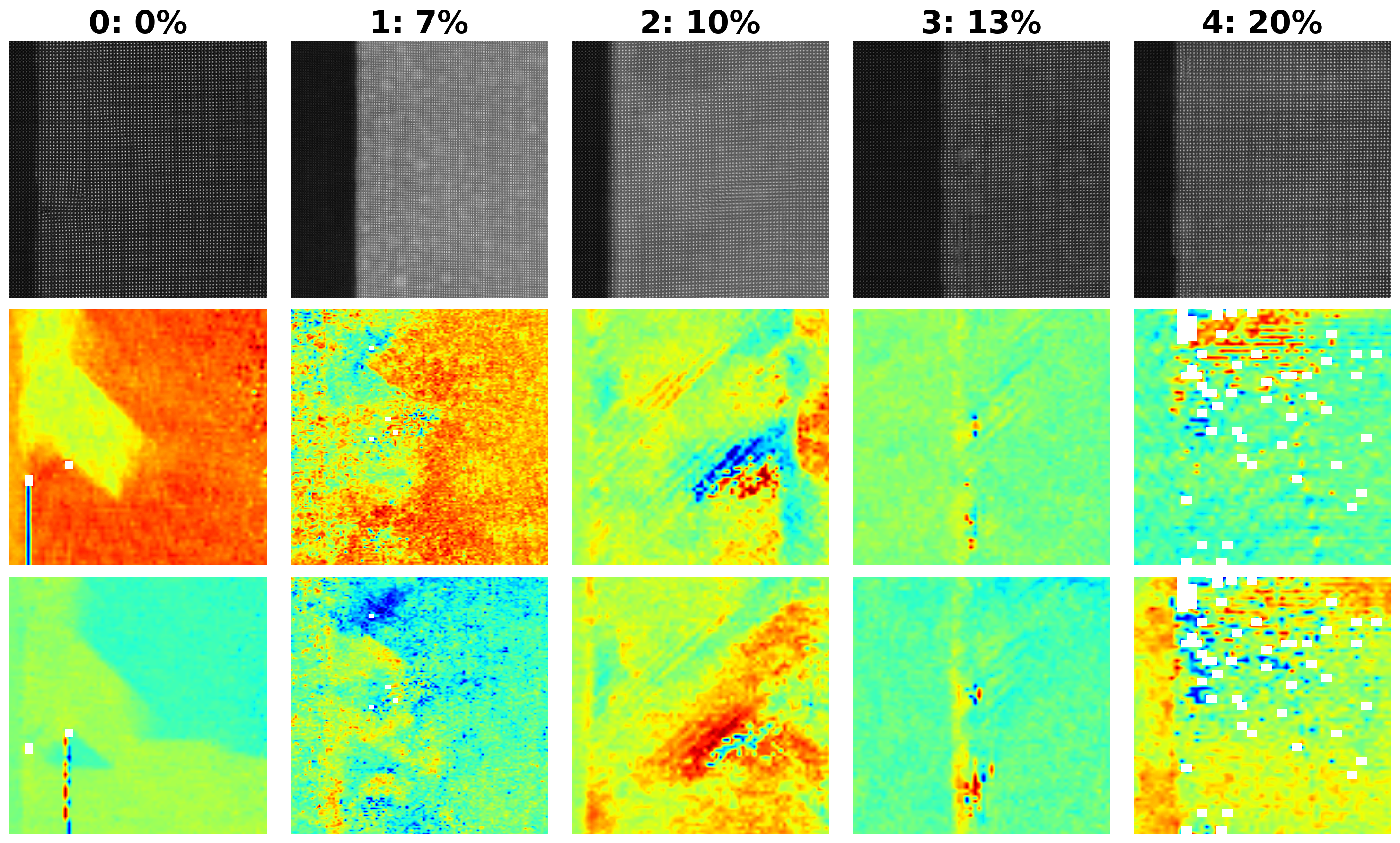
As you can see, this carefully curated dataset provides access to the raw imaging data and to the order parameter fields including poalrization components, strains, unit cell parameters, column intensities, and so on. The data set was curated to explude regions around defects.
Select a part of the image to save time in analysis
# Let's create new lists to store the selected images, Px, and Py data
selected_images = []
ground_truth_px = []
ground_truth_py = []

# Define the main area to be highlighted
main = [1000, 3000, 400, 2400]  # [y_start, y_end, x_start, x_end]

# Loop over the selected indices, extract the region, and store it
for i in np.arange(imnum):
    k = SBFOdata[i]

    # Select the region from the image, Px, and Py
    selected_image = k['Image'][main[0]:main[1], main[2]:main[3]]
    selected_px = k['ab_Px_resized'][main[0]:main[1], main[2]:main[3]]
    selected_py = k['ab_Py_resized'][main[0]:main[1], main[2]:main[3]]

    # Append the selected regions to the corresponding lists
    selected_images.append(selected_image)
    ground_truth_px.append(selected_px)
    ground_truth_py.append(selected_py)

# The selected images, ground truth Px, and ground truth Py have been stored in the lists:
# selected_images, ground_truth_px, and ground_truth_py
# I will now display a confirmation of the stored data.
len(selected_images), len(ground_truth_px), len(ground_truth_py)
(5, 5, 5)Define function for analysis
# min-max normalization:
def norm2d(img: np.ndarray) -> np.ndarray:
    return (img - np.min(img)) / (np.max(img) - np.min(img))
def custom_extract_subimages(imgdata, coordinates, w_prime):
# Stage 1: Extract subimages with a fixed size (64x64)
large_window_size = (64, 64)
half_height_large = large_window_size[0] // 2
half_width_large = large_window_size[1] // 2
subimages_largest = []
coms_largest = []
for coord in coordinates:
cx = int(np.around(coord[0]))
cy = int(np.around(coord[1]))
top = max(cx - half_height_large, 0)
bottom = min(cx + half_height_large, imgdata.shape[0])
left = max(cy - half_width_large, 0)
right = min(cy + half_width_large, imgdata.shape[1])
subimage = imgdata[top:bottom, left:right]
if subimage.shape[0] == large_window_size[0] and subimage.shape[1] == large_window_size[1]:
subimages_largest.append(subimage)
coms_largest.append(coord)
# Stage 2: Use these centers to extract subimages of window size `w1`
half_height = w_prime[0] // 2
half_width = w_prime[1] // 2
subimages_target = []
coms_target = []
for coord in coms_largest:
cx = int(np.around(coord[0]))
cy = int(np.around(coord[1]))
top = max(cx - half_height, 0)
bottom = min(cx + half_height, imgdata.shape[0])
left = max(cy - half_width, 0)
right = min(cy + half_width, imgdata.shape[1])
subimage = imgdata[top:bottom, left:right]
if subimage.shape[0] == w_prime[0] and subimage.shape[1] == w_prime[1]:
subimages_target.append(subimage)
coms_target.append(coord)
return np.array(subimages_target), np.array(coms_target)def build_descriptor(window_size, min_sigma, max_sigma, threshold, overlap):
processed_img = img
all_atoms = skimage.feature.blob_log(processed_img, min_sigma, max_sigma, 30, threshold, overlap)
coordinates = all_atoms[:, : -1]
# Extract subimages
subimages_target, coms_target = custom_extract_subimages(processed_img, coordinates, window_size)
# Build descriptors
descriptors = [subimage.flatten() for subimage in subimages_target]
descriptors = np.array(descriptors)
return descriptors, coms_target, all_atoms, coordinates, subimages_target# Define the Fit_GMM_param function without PCA, including covariance type
def Fit_GMM(descriptors, components, covariance_type):
# First pass of GMM to estimate initial parameters
# Flatten each subimage into a 1D vector
flattened_descriptors = descriptors.reshape(descriptors.shape[0], -1)
# Remove subimages with NaN values
mask = ~np.isnan(flattened_descriptors).any(axis=1)
valid_subimages = flattened_descriptors[mask]
preliminary_gmm = GaussianMixture(n_components=components, covariance_type=covariance_type, random_state=42)
preliminary_gmm.fit(valid_subimages)
initial_means = preliminary_gmm.means_
initial_weights = preliminary_gmm.weights_
# Initialize and fit the GMM using the parameters from the preliminary GMM
gmm = GaussianMixture(n_components=components,
means_init=initial_means,
weights_init=initial_weights,
covariance_type=covariance_type,
random_state=42)
gmm.fit(valid_subimages)
# Map the labels back to the original data, including NaN-handling
labels = gmm.predict(valid_subimages)
full_labels = np.full(valid_subimages.shape[0], -1)
full_labels[mask] = labels
return labels, valid_subimagesdef Fit_PCA_GMM(descriptors, n_clusters, components, covariance_type):
# Flatten each subimage into a 1D vector
flattened_descriptors = descriptors.reshape(descriptors.shape[0], -1)
# Remove subimages with NaN values
mask = ~np.isnan(flattened_descriptors).any(axis=1)
valid_subimages = flattened_descriptors[mask]
# Apply PCA for dimensionality reduction
pca = PCA(n_components=n_clusters)
reduced_data = pca.fit_transform(valid_subimages)
# Fit the preliminary GMM using valid subimages (without NaN values)
preliminary_gmm = GaussianMixture(n_components=components, covariance_type=covariance_type, random_state=42)
preliminary_gmm.fit(reduced_data)
initial_means = preliminary_gmm.means_
initial_weights = preliminary_gmm.weights_
# Initialize the GMM with the parameters from the preliminary fit
gmm = GaussianMixture(n_components=components,
means_init=initial_means,
weights_init=initial_weights,
covariance_type=covariance_type,
random_state=42)
gmm.fit(reduced_data)
# Predict labels for the valid subimages
labels = gmm.predict(reduced_data)
# Map the labels back to the original data, including NaN-handling
full_labels = np.full(flattened_descriptors.shape[0], -1) # Initialize full labels with -1
full_labels[mask] = labels # Only set labels for valid subimages
return full_labels, reduced_dataSelect Image of Interest
In this analysis, we focus on a selected STEM image from a larger dataset.
Detecting Atomic Features in the STEM image using the blob_log function from skimage.feature identifies potential atomic positions using a Laplacian of Gaussian (LoG) approach.
Extracting Subimages: using the detected coordinates, the function custom_extract_subimages is called to generate fixed-size subimages around each detected atomic feature.
Flattening Subimages for Descriptor Generation: Each subimage is flattened into a one-dimensional array, creating a consistent descriptor format for further analysis or machine learning applications.
import pickle# ! gdown --fuzzy --id 1AHlk5xxXiuiTtYNr8fk0YQ8Uxjbf8bfT
# Load the lists from the pickle file
images_data = "images_data.pkl"
with open(images_data, "rb") as f:
selected_images, ground_truth_px, ground_truth_py = pickle.load(f)
# Confirm successful loading by checking the lengths of the lists
print(len(selected_images), len(ground_truth_px), len(ground_truth_py))5 5 5
image = selected_images[0]
img = norm2d(image)
example descriptor to test
window_size = (40,40)
min_sigma = 1
max_sigma = 5
threshold = 0.025
overlap = 0.0
descriptors, coms_target, all_atoms, coordinates, subimages_target = build_descriptor(window_size, min_sigma, max_sigma, threshold, overlap)
print(descriptors.shape)
print(coms_target.shape)
print(all_atoms.shape)
print(coordinates.shape)
print(subimages_target.shape)(10917, 1600)
(10917, 2)
(11813, 3)
(11813, 2)
(10917, 40, 40)
Descriptor Visualization
plt.figure(figsize=(6, 6))
plt.imshow(image, cmap='gray')
plt.scatter(coms_target[:, 1], coms_target[:, 0], c='r', marker='o', s = 20
)
plt.axis('off')
plt.title('Image with Subimage Centers')
plt.xlim([300, 700])
plt.ylim([300, 700])
plt.show()
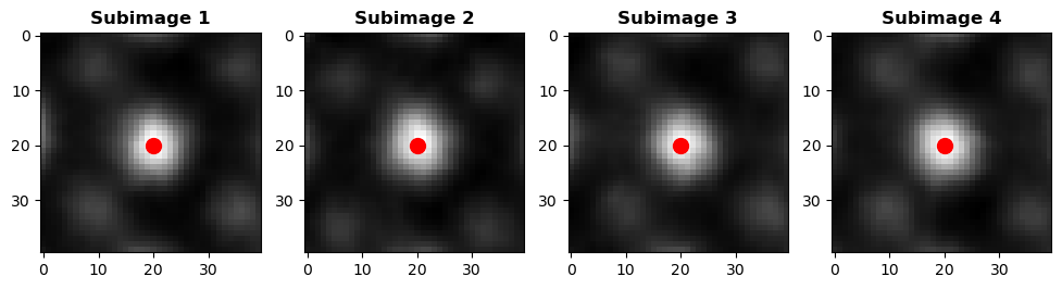
# Plot a few example subimages with their centers
fig, axes = plt.subplots(1, 4, figsize=(12, 3))
for i, ax in enumerate(axes):
ax.imshow(subimages_target[i], cmap='gray')
ax.scatter(window_size[1] // 2, window_size[0] // 2, c='r', marker='o', s = 100)
ax.set_title(f'Subimage {i+1}', fontweight = "bold")
plt.show()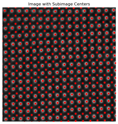
Average descriptor of all subimages
# Calculate and visualize the average descriptor
average_descriptor = descriptors.mean(axis=0).reshape(window_size)
plt.figure(figsize=(6, 6))
plt.imshow(average_descriptor, cmap='viridis')
plt.colorbar()
plt.title("Average Descriptor of All Subimages")
# plt.axis('off')
plt.show()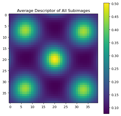
Here, we’re applying clustering to the descriptors extracted from subimages to group similar structural features and then visualizing the clusters to better understand the patterns in the data.
Clustering with Gaussian Mixture Model (GMM)
GMM on Raw Descriptors (Fit_GMM):
The function Fit_GMM is applied directly to the descriptors, with 5 clusters specified and a “full” covariance type. This model assumes the data can be represented by a mixture of 5 Gaussian distributions with unrestricted covariance matrices (i.e., allowing each cluster to have its unique shape).
Outputs: labels: Cluster labels assigned to each subimage, indicating the group each subimage belongs to.
valid_subimages: The subset of descriptors that were successfully clustered.
PCA and GMM Combined (Fit_PCA_GMM):
The Fit_PCA_GMM function applies Principal Component Analysis (PCA) to reduce the dimensionality of the descriptors from high-dimensional space down to 2 principal components (PCs).
labels, valid_subimages = Fit_GMM(descriptors, 5, "full")labels_pca, reduced_data_pca = Fit_PCA_GMM(descriptors, 2, 5, "full")fig , axes = plt.subplots(1, 2 , figsize = (12, 5))
axes[0].scatter(valid_subimages[:, 0], valid_subimages[:, 1], c=labels, s=20, cmap='jet', edgecolor='k')
axes[0].set_title('GMM clustering' , fontsize = 16, fontweight = "bold")
axes[0].set_xlabel('C1')
axes[0].set_ylabel('C2')
axes[1].scatter(reduced_data_pca[:, 0], reduced_data_pca[:, 1], c=labels_pca, s=20, cmap='jet', edgecolor='k')
axes[1].set_title('GMM PCA clustering' , fontsize = 16, fontweight = "bold")
axes[1].set_xlabel('PC1')
axes[1].set_ylabel('PC2')
plt.show()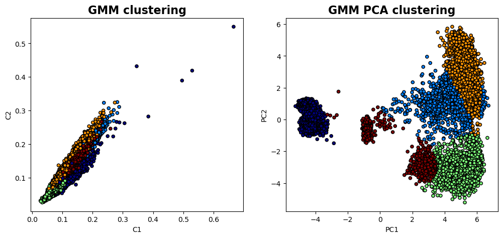
GMM Clustering on Raw Descriptors: Shows how the data clusters naturally in the full feature space, revealing groups based on subtle structural differences.
PCA-Reduced Clustering: Highlights patterns in the data’s most significant variance directions, simplifying the feature space and often revealing clearer group separations.
The visualization below depicts the centroids and dispersions of clusters, providing insights into their central tendencies and variability.
- The centroids, representing the mean values of descriptors within each cluster, highlight key features distinct to each cluster.
- The dispersions illustrate the standard deviations of the descriptors, indicating the degree of variability among cluster members. Together, these visualizations reveal both the characteristic features and the stability of each cluster.
# Initialize lists to store the centroids and dispersions
cluster_centroids = []
cluster_dispersions = []

# Calculate the overall mean descriptor
overall_mean = descriptors.mean(axis=0)

# Calculate the centroids and dispersions for each cluster
for cluster_label in np.unique(labels):
    # Get descriptors for the current cluster
    cluster_descriptors = descriptors[labels == cluster_label]
    # Calculate centroid and dispersion (standard deviation) for each cluster
    centroid = cluster_descriptors.mean(axis=0) - overall_mean
    dispersion = cluster_descriptors.std(axis=0)
    # Append results
    cluster_centroids.append(centroid)
    cluster_dispersions.append(dispersion)

# Convert to NumPy arrays for easy handling
cluster_centroids = np.array(cluster_centroids)
cluster_dispersions = np.array(cluster_dispersions)

# Plot the centroids and dispersions
fig, axes = plt.subplots(2, len(cluster_centroids), figsize=(15, 10))

# First row: Cluster centroids (centered)
for i, ax in enumerate(axes[0]):
    centroid_image = cluster_centroids[i].reshape(window_size)
    im_centroid = ax.imshow(centroid_image, cmap='coolwarm', aspect='auto')
    ax.set_title(f'Cluster {i+1} Centroid', fontweight="bold")
    ax.axis('off')

# Second row: Cluster dispersions (standard deviation within each cluster)
for i, ax in enumerate(axes[1]):
    dispersion_image = cluster_dispersions[i].reshape(window_size)
    im_dispersion = ax.imshow(dispersion_image, cmap='viridis', aspect='auto')
    ax.set_title(f'Cluster {i+1} Dispersion', fontweight="bold")
    ax.axis('off')

# # Add colorbars for interpretation
# fig.colorbar(im_centroid, ax=axes[0], orientation='vertical', fraction=0.02, pad=0.04)
# fig.colorbar(im_dispersion, ax=axes[1], orientation='vertical', fraction=0.02, pad=0.04)

plt.suptitle("Cluster Centroids and Dispersion (Standard Deviation) Across Descriptors", fontsize=16, fontweight="bold")
plt.tight_layout()
plt.show()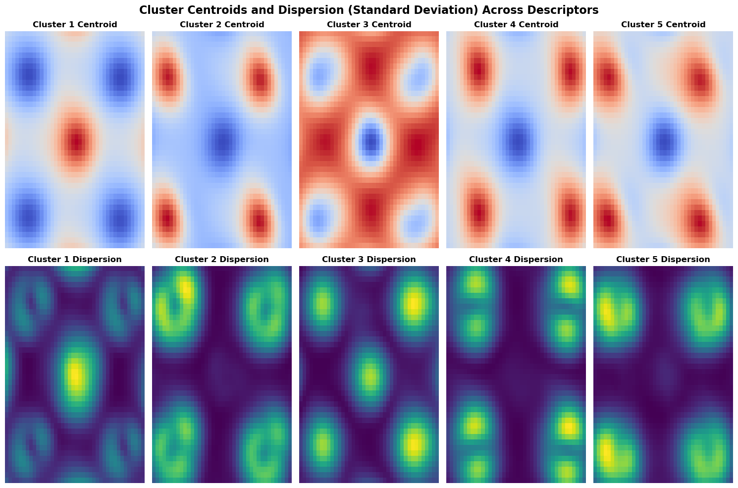
fig, ax = plt.subplots(1, 2, figsize=(12, 5))

# First subplot
ax[0].scatter(coms_target[:, 1], coms_target[:, 0], c=labels, s=10, cmap='jet', marker="s")
ax[0].set_title('GMM' , fontsize = 16, fontweight = "bold")
ax[0].axis('off')

ax[1].scatter(coms_target[:, 1], coms_target[:, 0], c=labels_pca, s=10, cmap='jet', marker="s")
ax[1].set_title('PCA GMM' , fontsize = 16, fontweight = "bold")
ax[1].axis('off')  # Just to leave it empty for now

plt.show()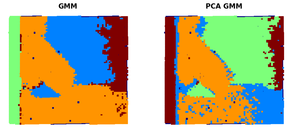
# Interactive function for plotting
def interactive_gmm_pca(window_width, window_height):
    # Parameters
    window_size = (window_width, window_height)
    min_sigma = 1
    max_sigma = 5
    threshold = 0.025
    overlap = 0.0

    # Build descriptors and fit models
    descriptors, coms_target, _, _, _ = build_descriptor(window_size, min_sigma, max_sigma, threshold, overlap)
    labels, valid_subimages = Fit_GMM(descriptors, 5, "full")
    labels_pca, reduced_data_pca = Fit_PCA_GMM(descriptors, 2, 5, "full")

    # Create a 2x2 plot
    fig, axes = plt.subplots(2, 2, figsize=(12, 12))

    # GMM Clusters
    axes[0, 0].scatter(valid_subimages[:, 0], valid_subimages[:, 1], c=labels, s=20, cmap='jet', edgecolor='k')
    axes[0, 0].set_title('GMM Clusters', fontsize=16, fontweight="bold")
    axes[0, 0].set_xlabel('C1')
    axes[0, 0].set_ylabel('C2')

    # PCA Clusters
    axes[0, 1].scatter(reduced_data_pca[:, 0], reduced_data_pca[:, 1], c=labels_pca, s=20, cmap='jet', edgecolor='k')
    axes[0, 1].set_title('PCA GMM Clusters', fontsize=16, fontweight="bold")
    axes[0, 1].set_xlabel('PC1')
    axes[0, 1].set_ylabel('PC2')

    # GMM Final Maps
    axes[1, 0].scatter(coms_target[:, 1], coms_target[:, 0], c=labels, s=10, cmap='jet', marker="s")
    axes[1, 0].set_title('GMM Final Map', fontsize=16, fontweight="bold")
    axes[1, 0].axis('off')

    # PCA Final Maps
    axes[1, 1].scatter(coms_target[:, 1], coms_target[:, 0], c=labels_pca, s=10, cmap='jet', marker="s")
    axes[1, 1].set_title('PCA Final Map', fontsize=16, fontweight="bold")
    axes[1, 1].axis('off')

    # Adjust layout
    plt.tight_layout()
    plt.show()
# fig_gmm_widget_1
import ipywidgets
ipywidgets.interact(interactive_gmm_pca,
window_width=widgets.IntSlider(min=2, max=64, step=2, value=2, description='Width'),
window_height=widgets.IntSlider(min=2, max=64, step=2, value=2, description='Height'))<function __main__.interactive_gmm_pca(window_width, window_height)>As you can see, the use of the GMM clustering in the original descriptor space (i.e. 1600 dimensional space if the descriptor is 40x40 image patch) gives a pretty good separation of several domain configurations and substrate. The GMM clustering of the data set that was dimensionality reduced by PCA shows additional details - for example, you can see that the domain on the bottom is now split in two parts. Practically, it happens because the STEM imaging is not ideal, and the image suffers from mis-tilt effect (small deviation of the column direction from the beam direction). Npte that this mistilt effect is not visible on the polarization field maps. So we can start asking questions like:
- What is the “right” way to analyze the data?
- What other information on materials properties is hidden in the images?
- And how can we extract it combining both the data-driven and physical insights?
Let’s explore this using the VAE approaches!
VAE
Now, let’s explore our imaging data using the simple VAE.
The Variational Autoencoder (VAE) is a type of deep generative model that can learn to encode high-dimensional data, such as images, into a low-dimensional latent space and then decode that latent representation back to the original data space. A VAE is particularly useful in imaging data, as it can capture meaningful features in a compressed form, making it easier to analyze patterns, generate new images, or explore variations in the data.
What Does a Simple VAE Do?
Encoder:
The encoder maps the input image into a latent space by compressing it into a lower-dimensional representation. Unlike a traditional autoencoder, which might produce a fixed vector, the VAE encoder outputs two components for each latent dimension: a mean and a log variance. These parameters define a Gaussian distribution over the latent space for each input.
Latent Space Sampling:
After the encoder produces a mean and variance, a sample is drawn from this Gaussian distribution, which allows the VAE to introduce some randomness or variability into the latent representation. The sampling process makes the VAE a generative model, enabling it to create new images by sampling different points in the latent space.
Decoder:
The sampled latent vector is then fed to the decoder, which reconstructs the image. The decoder tries to reproduce the original input as accurately as possible, allowing the VAE to learn a compressed, yet informative, representation of the input data.
Loss Function:
The VAE optimizes two components: Reconstruction Loss: Measures the similarity between the input image and the reconstructed image, encouraging the VAE to accurately capture image details. KL Divergence: Regularizes the latent space, ensuring the learned latent distributions are close to a standard Gaussian. This keeps the latent space smooth, meaning that similar points in the latent space correspond to similar reconstructed images.
First, let’s prepare the data:
#normalize imagestack
subimages_target = subimages_target/subimages_target.max()
subimages_target = np.expand_dims(subimages_target, axis=-1)
train_data = torch.tensor(subimages_target[:,:,:,0]).float()
train_loader = pv.utils.init_dataloader(train_data.unsqueeze(1), batch_size=48, seed=0)
Now, running the VAE in PyroVEd. Simple VAE will find the best representation of our data as two components for latent vecotr (l1,l2). Of course, we can explore other dimensinalities of latent space!
in_dim = (window_size[0],window_size[1])

# Initialize vanilla VAE
vae = pv.models.iVAE(in_dim, latent_dim=2,   # Number of latent dimensions other than the invariancies
                     hidden_dim_e = [512, 512],
                     hidden_dim_d = [512, 512], # corresponds to the number of neurons in the hidden layers of the decoder
                     invariances=None, seed=0)
# Initialize SVI trainer
trainer = pv.trainers.SVItrainer(vae)

# Train for n epochs:
for e in range(10):
    trainer.step(train_loader)
    trainer.print_statistics()
Epoch: 1 Training loss: 698.3063
Epoch: 2 Training loss: 677.7180
Epoch: 3 Training loss: 676.9961
Epoch: 4 Training loss: 676.6272
Epoch: 5 Training loss: 676.3806
Epoch: 6 Training loss: 676.6844
Epoch: 7 Training loss: 676.5142
Epoch: 8 Training loss: 676.2313
Epoch: 9 Training loss: 676.3100
Epoch: 10 Training loss: 675.8797
Varitional Auto Encoder manifold representation
vae_laten_img = vae.manifold2d(d=10, draw_grid = True, origin = 'lower')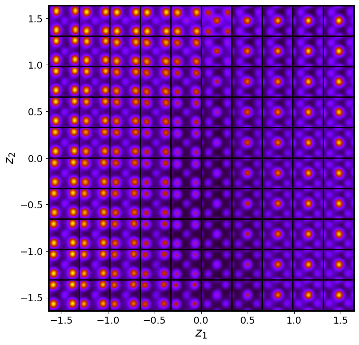
The latent representation of the system is visualized as a grid over the two latent variables and . Each grid cell corresponds to a unique combination of values for and , which are decoded to produce corresponding reconstructions in the data space. The smooth and structured transition across the grid indicates that the model has learned a meaningful and continuous mapping between the latent variables and the data space. Variations in the grid reflect changes in the underlying physical structure, such as column type, domain orientation, or material properties.
vae_z_mean, vae_z_sd = vae.encode(train_data)
z1 = vae_z_mean[:, -2]
z2 = vae_z_mean[:, -1]
Latent representation
# Plot
plt.figure(figsize=(6, 6), facecolor='white', dpi=200)

# Scatterplot
plt.scatter(z1, z2, s=15, edgecolor='k', linewidth=0.5, alpha=0.4, c="b")

# KDE plot
sns.kdeplot(x=z1, y=z2, cmap="Oranges", levels=50, thresh=0.005, alpha=0.5, fill=True)

# Labels and title
plt.xlabel(r"$z_1$", fontsize=14)
plt.ylabel(r"$z_2$", fontsize=14)
plt.title("KDE with Scatter", fontsize=16)

plt.tight_layout()
plt.show()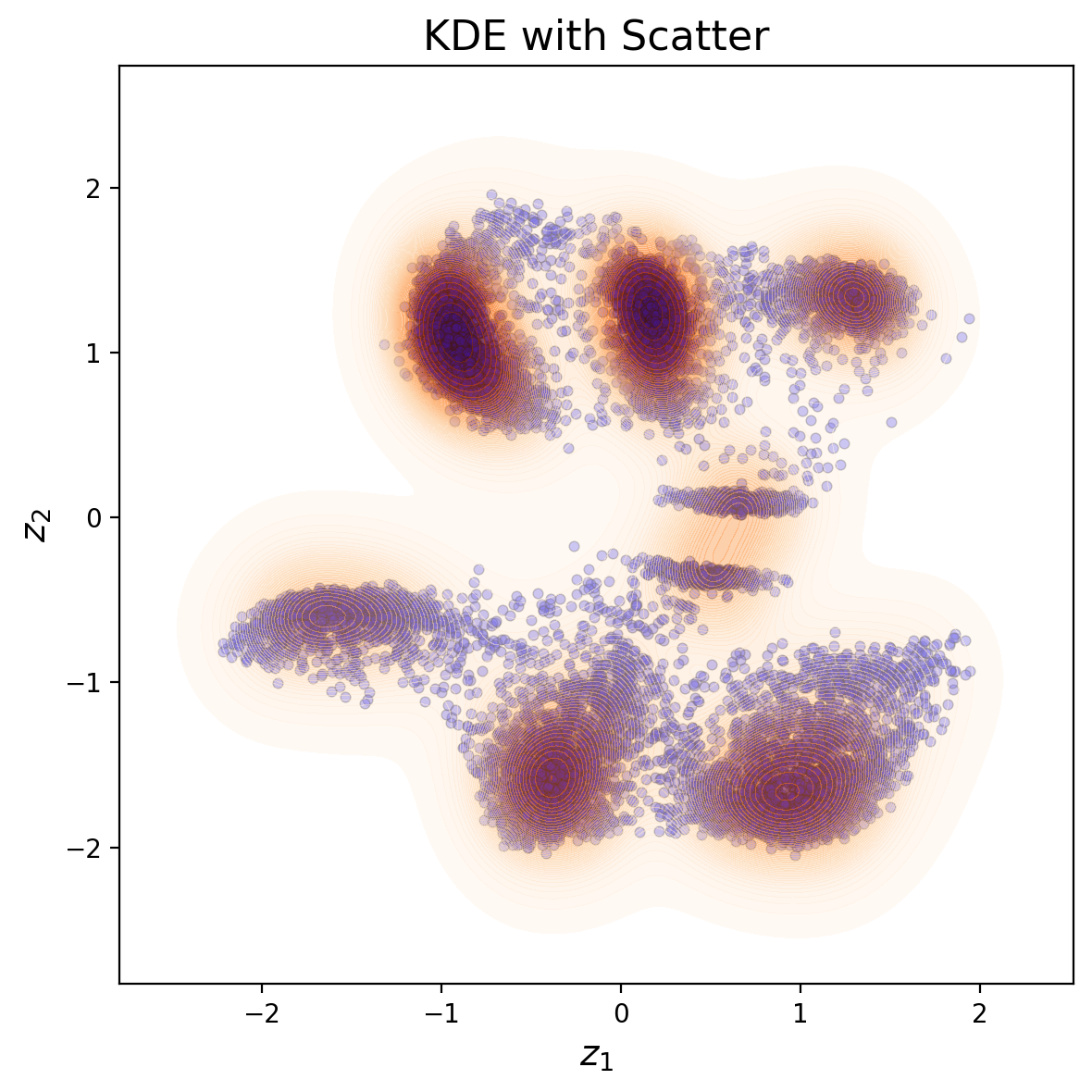
def generate_latent_manifold(n=10, decoder=None, target_size=(28, 28)):
    """
    Generate a general latent manifold grid over the entire latent space.
    """
    # Define grid bounds across latent space
    grid_x = np.linspace(min(z1), max(z1), n)
    grid_y = np.linspace(min(z2), max(z2), n)

    # Dynamically infer output shape
    sample_input = torch.tensor([[grid_x[0], grid_y[0]]], dtype=torch.float32)
    with torch.no_grad():
        X_decoded = decoder(sample_input)
    decoded_shape = X_decoded.shape[-2:] if len(X_decoded.shape) > 2 else (X_decoded.shape[-1], X_decoded.shape[-1])

    height, width = target_size
    manifold = np.zeros((height * n, width * n))

    # Generate manifold
    for i, yi in enumerate(grid_x):
        for j, xi in enumerate(grid_y):
            Z_sample = torch.tensor([[xi, yi]], dtype=torch.float32)
            with torch.no_grad():
                X_decoded = decoder(Z_sample).reshape(decoded_shape)
            resized_image = zoom(X_decoded, zoom=(height / X_decoded.shape[-2], width / X_decoded.shape[-1]))
            manifold[i * height: (i + 1) * height, j * width: (j + 1) * width] = resized_image
    return manifold
# VAE_manifold_1
fig, axes = plt.subplots(1, 2, figsize=(12, 6))
# Generate and plot latent manifold
manifold = generate_latent_manifold(n=10, decoder=vae.decode, target_size=(28, 28))
axes[0].imshow(manifold, cmap="gnuplot2", origin="upper")
axes[0].set_xlabel(r"$z_1$", fontsize=16)
axes[0].set_ylabel(r"$z_2$", fontsize=16)
axes[0].set_xticks([])
axes[0].set_yticks([])
# Add "a)" to the first subplot
axes[0].text(-0.02, 1, 'a)', transform=axes[0].transAxes, fontsize=16, fontweight='bold', va='top', ha='right')
# Scatter and KDE plot using sns
sns.scatterplot(x=z1, y=z2, ax=axes[1], color="b", alpha=0.4, edgecolor="k", s=10)
sns.kdeplot(x=z1, y=z2, ax=axes[1], cmap="Oranges", levels=30, thresh=0.005, alpha=0.6, fill=True)
axes[1].set_xlabel(r"$z_1$", fontsize=16)
axes[1].set_ylabel(r"$z_2$", fontsize=16)
# Add "b)" to the second subplot
axes[1].text(-0.05, 1, 'b)', transform=axes[1].transAxes, fontsize=16, fontweight='bold', va='top', ha='right')
plt.tight_layout()
plt.show()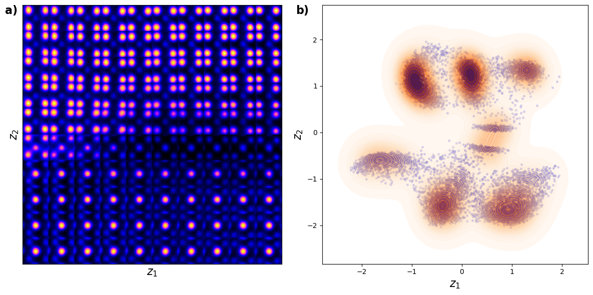
Shown above is the latent distirbution of the system
You can see selveral clusters in the latent space. These correspond to the column type (the primary factor of variation), ferroelectric domain orientation, and nature of material (BFO or substarte). Note that in this case all fatcors of variation are rperesented via just two latent variables.
Now, let’s explore the latent maps. Remember that each column have become two latent variables, so we can plot them in real space.
# Px = SBFOdata[0]["ab_Px_resized"][main[0]:main[1], main[2]:main[3]]  # Ground truth Px
# Py = SBFOdata[0]["ab_Py_resized"][main[0]:main[1], main[2]:main[3]]  # Ground truth Py

# def plot_all_variables(z1, z2, Px, Py, coms_target):
#     fig, axes = plt.subplots(2, 2, figsize=(12, 12))

#     # Plot z1
#     sc1 = axes[0, 0].scatter(coms_target[:, 1], coms_target[:, 0], c=z1, s=14, cmap='jet', marker="o")
#     axes[0, 0].set_title("z1", fontsize=16, fontweight = "bold")
#     # fig.colorbar(sc1, ax=axes[0, 0])
#     axes[0, 0].axis("off")

#     # Plot z2
#     sc2 = axes[0, 1].scatter(coms_target[:, 1], coms_target[:, 0], c=z2, s=14, cmap='jet', marker="o")
#     axes[0, 1].set_title("z2", fontsize=16, fontweight = "bold")
#     # fig.colorbar(sc2, ax=axes[0, 1])
#     axes[0, 1].axis("off")

#     # Plot Px
#     im1 = axes[1, 0].imshow(Px, cmap='jet', origin='lower')
#     axes[1, 0].set_title("Ground Truth Px", fontsize=16,  fontweight = "bold")
#     # fig.colorbar(im1, ax=axes[1, 0])
#     axes[1, 0].axis("off")

#     # Plot Py
#     im2 = axes[1, 1].imshow(Py, cmap='jet', origin='lower')
#     axes[1, 1].set_title("Ground Truth Py", fontsize=16, fontweight = "bold")
#     # fig.colorbar(im2, ax=axes[1, 1])
#     axes[1, 1].axis("off")

#     plt.tight_layout()
#     plt.show()
Px = SBFOdata[0]["ab_Px_resized"][main[0]:main[1], main[2]:main[3]] # Ground truth Px
Py = SBFOdata[0]["ab_Py_resized"][main[0]:main[1], main[2]:main[3]] # Ground truth Py
def plot_all_variables(z1, z2, Px, Py, coms_target):
fig, axes = plt.subplots(2, 2, figsize=(12, 12))
# Plot z1
sc1 = axes[0, 0].scatter(coms_target[:, 1], coms_target[:, 0], c=z1, s=14, cmap='jet', marker="o")
axes[0, 0].set_title("z1", fontsize=16, fontweight="bold")
axes[0, 0].text(-0.1, 1, 'a)', transform=axes[0, 0].transAxes, fontsize=16, fontweight='bold', va='top', ha='right')
axes[0, 0].axis("off")
# Plot z2
sc2 = axes[0, 1].scatter(coms_target[:, 1], coms_target[:, 0], c=z2, s=14, cmap='jet', marker="o")
axes[0, 1].set_title("z2", fontsize=16, fontweight="bold")
axes[0, 1].text(-0.1, 1, 'b)', transform=axes[0, 1].transAxes, fontsize=16, fontweight='bold', va='top', ha='right')
axes[0, 1].axis("off")
# Plot Px
im1 = axes[1, 0].imshow(Px, cmap='jet', origin='lower')
axes[1, 0].set_title("Ground Truth Px", fontsize=16, fontweight="bold")
axes[1, 0].text(-0.1, 1, 'c)', transform=axes[1, 0].transAxes, fontsize=16, fontweight='bold', va='top', ha='right')
axes[1, 0].axis("off")
# Plot Py
im2 = axes[1, 1].imshow(Py, cmap='jet', origin='lower')
axes[1, 1].set_title("Ground Truth Py", fontsize=16, fontweight="bold")
axes[1, 1].text(-0.1, 1, 'd)', transform=axes[1, 1].transAxes, fontsize=16, fontweight='bold', va='top', ha='right')
axes[1, 1].axis("off")
plt.tight_layout()
plt.show()# Latent_maps_1
plot_all_variables(z1, z2, Px, Py, coms_target)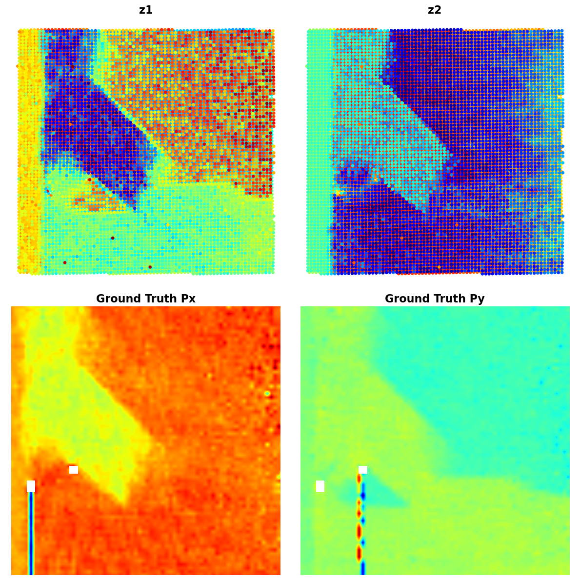
# Replace with your actual data
z1 = z1  # Latent variable 1
z2 = z2  # Latent variable 2
Px = SBFOdata[0]["ab_Px_resized"][main[0]:main[1], main[2]:main[3]]  # Ground truth Px
Py = SBFOdata[0]["ab_Py_resized"][main[0]:main[1], main[2]:main[3]]  # Ground truth Py
coms_target = coms_target  # Coordinates for scatter plots

# List of options
options = ["z1", "z2", "Ground Truth Px", "Ground Truth Py"]

# Function to plot two selected variables
def plot_two_variables(variable1, variable2):
    fig, axes = plt.subplots(1, 2, figsize=(12, 6))

    # Plot for variable 1
    if variable1 == "z1":
        axes[0].scatter(coms_target[:, 1], coms_target[:, 0], c=z1, s=14, cmap='jet', marker="o")
        axes[0].set_title("Latent Variable z1", fontsize=16)
    elif variable1 == "z2":
        axes[0].scatter(coms_target[:, 1], coms_target[:, 0], c=z2, s=14, cmap='jet', marker="o")
        axes[0].set_title("Latent Variable z2", fontsize=16)
    elif variable1 == "Ground Truth Px":
        axes[0].imshow(Px, cmap='jet', origin='lower')
        axes[0].set_title("Ground Truth Px", fontsize=16)
    elif variable1 == "Ground Truth Py":
        axes[0].imshow(Py, cmap='jet', origin='lower')
        axes[0].set_title("Ground Truth Py", fontsize=16)

    axes[0].axis("off")

    # Plot for variable 2
    if variable2 == "z1":
        axes[1].scatter(coms_target[:, 1], coms_target[:, 0], c=z1, s=14, cmap='jet', marker="o")
        axes[1].set_title("Latent Variable z1", fontsize=16)
    elif variable2 == "z2":
        axes[1].scatter(coms_target[:, 1], coms_target[:, 0], c=z2, s=14, cmap='jet', marker="o")
        axes[1].set_title("Latent Variable z2", fontsize=16)
    elif variable2 == "Ground Truth Px":
        axes[1].imshow(Px, cmap='jet', origin='lower')
        axes[1].set_title("Ground Truth Px", fontsize=16)
    elif variable2 == "Ground Truth Py":
        axes[1].imshow(Py, cmap='jet', origin='lower')
        axes[1].set_title("Ground Truth Py", fontsize=16)

    axes[1].axis("off")

    plt.tight_layout()
    plt.show()
# import ipywidgets
# ipywidgets.interact(plot_two_variables,
# variable1=widgets.Dropdown(options=options, description="Variable 1"),
# variable2=widgets.Dropdown(options=options, description="Variable 2"))
<function __main__.plot_two_variables(variable1, variable2)>Not bad! We can see that our VAE anaysis has visualzied the domains as different contrats level for the z1 and z2. We see the difference between the substarte and material, and on z2 image we see the mistilt effect that shows like gradient towards the r.h.s. of the image.
However, this analysis has two big problems:
- the latent variables do not have defined physical meaning. To be more precide, we can interpret them with the latent representation, but that’s pretty much it.
- How do we know how many latent variable to choose?
rVAE
Now, let’s experiment with rotationally invariant VAE. Here, we try to encode the data as latent vecotr and rotation vecotr. Whereas latent variables attempt to represent the intirnsic facotrs of variation, rotation has a well defined physical meaning. SO if we choose the rVAE with 2D latent space, we effectively have 3 latent variables - 2 regular and one that encodes the orientation of out descriptor. We have started to learn physics!
in_dim = (window_size[0],window_size[1])

# Initialize vanilla VAE
rvae = pv.models.iVAE(in_dim, latent_dim=2,   # Number of latent dimensions other than the invariancies
                     hidden_dim_e = [512, 512],
                     hidden_dim_d = [512, 512], # corresponds to the number of neurons in the hidden layers of the decoder
                     invariances=["r"], seed=0)
# Initialize SVI trainer
trainer = pv.trainers.SVItrainer(rvae)

# Train for n epochs:
for e in range(10):
    trainer.step(train_loader)
    trainer.print_statistics()

rvae.save_weights('rvae_model')
print("Model saved successfully.")
Epoch: 1 Training loss: 773.8497
Epoch: 2 Training loss: 709.7926
Epoch: 3 Training loss: 695.4158
Epoch: 4 Training loss: 689.5364
Epoch: 5 Training loss: 686.7692
Epoch: 6 Training loss: 684.9871
Epoch: 7 Training loss: 683.6735
Epoch: 8 Training loss: 683.7374
Epoch: 9 Training loss: 682.9053
Epoch: 10 Training loss: 682.3702
Model saved successfully.
Varitional Auto Encoder manifold representation
rvae_laten_img = rvae.manifold2d(d=10, draw_grid = True, origin = 'lower')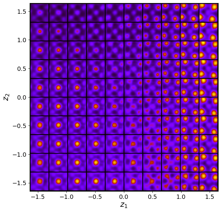
rvae_z_mean, rvae_z_sd = rvae.encode(train_data)
z1 = rvae_z_mean[:, -2]
z2 = rvae_z_mean[:, -1]
ang = rvae_z_mean[:, 0]
Latent representation
# fig_rVAE_widget_1


fig, axes = plt.subplots(2, 2, figsize=(12, 10))

# Define consistent axes limits
# z1_lim = [min(z1), max(z1)]
# z2_lim = [min(z2), max(z2)]
# ang_lim = [min(ang), max(ang)]

# (a) Latent manifold
manifold = generate_latent_manifold(n=10, decoder=rvae.decode, target_size=(28, 28))
axes[0, 0].imshow(manifold, cmap="gnuplot2", origin="upper", aspect='auto')
axes[0, 0].set_xlabel(r"$z_1$", fontsize=16)
axes[0, 0].set_ylabel(r"$z_2$", fontsize=16)
axes[0, 0].set_xticks([]), axes[0, 0].set_yticks([])
axes[0, 0].text(-0.05, 1, 'a)', transform=axes[0, 0].transAxes, fontsize=16, fontweight='bold', va='top', ha='right')

# (b) z1 vs z2 with KDE
sns.kdeplot(x=z1, y=z2, ax=axes[0, 1], cmap="Oranges", levels=30, fill=True, alpha=0.6, thresh=0.005)
sns.scatterplot(x=z1, y=z2, ax=axes[0, 1], color="b", s=10, alpha=0.4, edgecolor="k")
# axes[0, 1].set_xlim(z1_lim)
# axes[0, 1].set_ylim(z2_lim)
axes[0, 1].set_xlabel(r"$z_1$", fontsize=16, fontweight="bold")
axes[0, 1].set_ylabel(r"$z_2$", fontsize=16, fontweight="bold")
axes[0, 1].text(-0.05, 1, 'b)', transform=axes[0, 1].transAxes, fontsize=16, fontweight='bold', va='top', ha='right')

# (c) ang vs z2 with KDE
sns.kdeplot(x=ang, y=z2, ax=axes[1, 0], cmap="Oranges", levels=70, fill=True, alpha=0.6, thresh=0.005)
sns.scatterplot(x=ang, y=z2, ax=axes[1, 0], color="b", s=10, alpha=0.4, edgecolor="k")
# axes[1, 0].set_xlim(ang_lim)
# axes[1, 0].set_ylim(z2_lim)
axes[1, 0].set_xlabel("ang", fontsize=16, fontweight="bold")
axes[1, 0].set_ylabel(r"$z_2$", fontsize=16, fontweight="bold")
axes[1, 0].text(-0.05, 1, 'c)', transform=axes[1, 0].transAxes, fontsize=16, fontweight='bold', va='top', ha='right')

# (d) ang vs z1 with KDE
sns.kdeplot(x=ang, y=z1, ax=axes[1, 1], cmap="Oranges", levels=80, fill=True, alpha=0.6, thresh=0.005)
sns.scatterplot(x=ang, y=z1, ax=axes[1, 1], color="b", s=10, alpha=0.4, edgecolor="k")
# axes[1, 1].set_xlim(ang_lim)
# axes[1, 1].set_ylim(z1_lim)
axes[1, 1].set_xlabel("ang", fontsize=16, fontweight="bold")
axes[1, 1].set_ylabel(r"$z_1$", fontsize=16, fontweight="bold")
axes[1, 1].text(-0.05, 1, 'd)', transform=axes[1, 1].transAxes, fontsize=16, fontweight='bold', va='top', ha='right')

# Adjust layout and display
plt.tight_layout()
plt.show()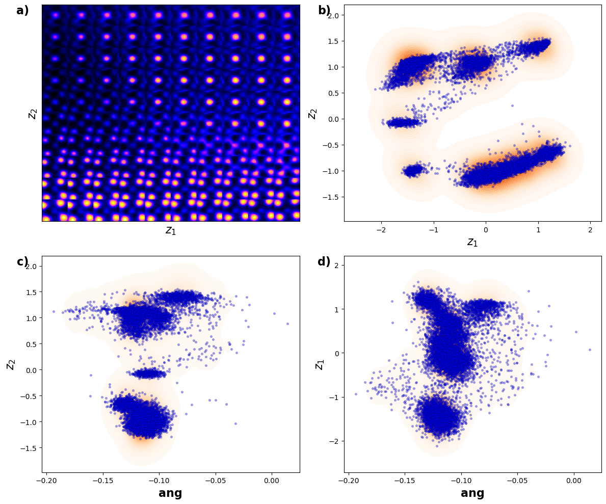
# # fig_rVAE_widget_1

# fig, axes = plt.subplots(2, 2, figsize=(12, 10))

# # Define consistent axes limits
# z1_lim = [min(z1), max(z1)]
# z2_lim = [min(z2), max(z2)]
# ang_lim = [min(ang), max(ang)]

# # (a) Latent manifold
# manifold = generate_latent_manifold(n=10, decoder=rvae.decode, target_size=(28, 28))
# axes[0, 0].imshow(manifold, cmap="gnuplot2", origin="upper", aspect='auto')
# axes[0, 0].set_xlabel(r"$z_1$", fontsize=16)
# axes[0, 0].set_ylabel(r"$z_2$", fontsize=16)
# axes[0, 0].set_xticks([]), axes[0, 0].set_yticks([])
# axes[0, 0].text(-0.05, 1, 'a)', transform=axes[0, 0].transAxes, fontsize=16, fontweight='bold', va='top', ha='right')

# # (b) z1 vs z2 with KDE
# kde = gaussian_kde([z1, z2])
# X, Y = np.meshgrid(np.linspace(*z1_lim, 200), np.linspace(*z2_lim, 200))
# Z = kde(np.vstack([X.ravel(), Y.ravel()])).reshape(X.shape)
# levels = np.linspace(Z.min() + 0.2 * (Z.max() - Z.min()), Z.max(), 30)  # Explicit levels

# axes[0, 1].contourf(X, Y, Z, levels=levels, cmap="jet", alpha=0.2)
# axes[0, 1].scatter(z1, z2, c="black", s=10, alpha=0.4, edgecolors="k")
# axes[0, 1].set_xlim(z1_lim), axes[0, 1].set_ylim(z2_lim)
# axes[0, 1].set_xlabel(r"$z_1$", fontsize=16)
# axes[0, 1].set_ylabel(r"$z_2$", fontsize=16)
# axes[0, 1].text(-0.05, 1, 'b)', transform=axes[0, 1].transAxes, fontsize=16, fontweight='bold', va='top', ha='right')

# # (c) ang vs z2 with KDE
# kde = gaussian_kde([ang, z2])
# X, Y = np.meshgrid(np.linspace(*ang_lim, 200), np.linspace(*z2_lim, 200))
# Z = kde(np.vstack([X.ravel(), Y.ravel()])).reshape(X.shape)
# levels = np.linspace(Z.min() + 0.2 * (Z.max() - Z.min()), Z.max(), 30)

# axes[1, 0].contourf(X, Y, Z, levels=levels, cmap="jet", alpha=0.2)
# axes[1, 0].scatter(ang, z2, c="black", s=10, alpha=0.4, edgecolors="k")
# axes[1, 0].set_xlim(ang_lim), axes[1, 0].set_ylim(z2_lim)
# axes[1, 0].set_xlabel("ang", fontsize=16)
# axes[1, 0].set_ylabel(r"$z_2$", fontsize=16)
# axes[1, 0].text(-0.05, 1, 'c)', transform=axes[1, 0].transAxes, fontsize=16, fontweight='bold', va='top', ha='right')

# # (d) ang vs z1 with KDE
# kde = gaussian_kde([ang, z1])
# X, Y = np.meshgrid(np.linspace(*ang_lim, 200), np.linspace(*z1_lim, 200))
# Z = kde(np.vstack([X.ravel(), Y.ravel()])).reshape(X.shape)
# levels = np.linspace(Z.min() + 0.2 * (Z.max() - Z.min()), Z.max(), 30)

# axes[1, 1].contourf(X, Y, Z, levels=levels, cmap="jet", alpha=0.2)
# axes[1, 1].scatter(ang, z1, c="black", s=10, alpha=0.4, edgecolors="k")
# axes[1, 1].set_xlim(ang_lim), axes[1, 1].set_ylim(z1_lim)
# axes[1, 1].set_xlabel("ang", fontsize=16)
# axes[1, 1].set_ylabel(r"$z_1$", fontsize=16)
# axes[1, 1].text(-0.05, 1, 'd)', transform=axes[1, 1].transAxes, fontsize=16, fontweight='bold', va='top', ha='right')

# # Adjust layout and display
# plt.tight_layout()
# plt.show()
Now, the clusters in latent space become more separated. These clearly correspond to the A- and B type cations now.
def plot_all_variables():
    fig, axes = plt.subplots(2, 3, figsize=(18, 12))

    # z1 plot
    scatter = axes[0, 0].scatter(coms_target[:, 1], coms_target[:, 0], c=z1, s=10, cmap='jet', marker="s")
    axes[0, 0].set_title("z1", fontsize=16, fontweight="bold")
    axes[0, 0].text(-0.01, 1, 'a)', transform=axes[0, 0].transAxes, fontsize=16, fontweight='bold', va='top', ha='right')
    axes[0, 0].axis("off")

    # z2 plot
    scatter = axes[0, 1].scatter(coms_target[:, 1], coms_target[:, 0], c=z2, s=10, cmap='jet', marker="s")
    axes[0, 1].set_title("z2", fontsize=16, fontweight="bold")
    axes[0, 1].text(-0.01, 1, 'b)', transform=axes[0, 1].transAxes, fontsize=16, fontweight='bold', va='top', ha='right')
    axes[0, 1].axis("off")

    # ang plot
    scatter = axes[0, 2].scatter(coms_target[:, 1], coms_target[:, 0], c=ang, s=10, cmap='jet', marker="s")
    axes[0, 2].set_title("ang", fontsize=16, fontweight="bold")
    axes[0, 2].text(-0.01, 1, 'c)', transform=axes[0, 2].transAxes, fontsize=16, fontweight='bold', va='top', ha='right')
    axes[0, 2].axis("off")

    # Px plot
    im = axes[1, 0].imshow(Px, cmap='jet', origin='lower')
    axes[1, 0].set_title("Ground Truth Px", fontsize=16, fontweight="bold")
    axes[1, 0].text(-0.01, 1, 'd)', transform=axes[1, 0].transAxes, fontsize=16, fontweight='bold', va='top', ha='right')
    axes[1, 0].axis("off")

    # Py plot
    im = axes[1, 1].imshow(Py, cmap='jet', origin='lower')
    axes[1, 1].set_title("Ground Truth Py", fontsize=16, fontweight="bold")
    axes[1, 1].text(-0.01, 1, 'e)', transform=axes[1, 1].transAxes, fontsize=16, fontweight='bold', va='top', ha='right')
    axes[1, 1].axis("off")

    # Remove unused axes
    axes[1, 2].axis("off")

    plt.tight_layout()
    plt.show()
# fig_rVAE_widget_2
plot_all_variables()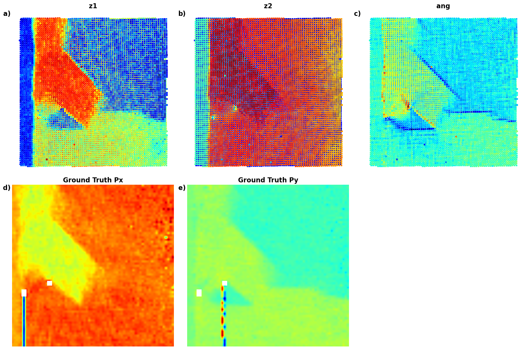
# import numpy as np
# import matplotlib.pyplot as plt
# from scipy.stats import gaussian_kde
# import ipywidgets as widgets
# from ipywidgets import interact

# # Define the data
# z1 = z1  # Latent variable 1
# z2 = z2  # Latent variable 2
# ang = ang  # Angular variable
# Px = SBFOdata[0]["ab_Px_resized"][main[0]:main[1], main[2]:main[3]]  # Ground truth Px
# Py = SBFOdata[0]["ab_Py_resized"][main[0]:main[1], main[2]:main[3]]  # Ground truth Py

# coms_target = coms_target  # Coordinates for scatter plots

# # Define options and data dictionary
# options = ["z1", "z2", "ang", "Ground Truth Px", "Ground Truth Py"]
# data_dict = {
#     "z1": z1,
#     "z2": z2,
#     "ang": ang,
#     "Ground Truth Px": Px,
#     "Ground Truth Py": Py
# }

# # Interactive function for plotting two selected variables
# def interactive_plot(variable1, variable2):
#     fig, axes = plt.subplots(1, 2, figsize=(12, 6))

#     # Plot for variable 1
#     values1 = data_dict[variable1]
#     if variable1 in ["z1", "z2", "ang"]:
#         scatter = axes[0].scatter(coms_target[:, 1], coms_target[:, 0], c=values1, s=10, cmap='jet', marker="s")
#     else:
#         im = axes[0].imshow(values1, cmap='jet', origin='lower')
#     axes[0].set_title(variable1, fontsize=16)
#     axes[0].axis("off")

#     # Plot for variable 2
#     values2 = data_dict[variable2]
#     if variable2 in ["z1", "z2", "ang"]:
#         scatter = axes[1].scatter(coms_target[:, 1], coms_target[:, 0], c=values2, s=10, cmap='jet', marker="s")
#     else:
#         im = axes[1].imshow(values2, cmap='jet', origin='lower')
#     axes[1].set_title(variable2, fontsize=16)
#     axes[1].axis("off")

#     plt.tight_layout()
#     plt.show()
# ipywidgets.interact(interactive_plot,
#          variable1=widgets.Dropdown(options=options, description="Variable 1"),
#          variable2=widgets.Dropdown(options=options, description="Variable 2"));
Latent maps
# data = [
#     (z1, "z1"),
#     (z2, "z2"),
#     (ang, "ang"),
#     (SBFOdata[1]["ab_Px_resized"][main[0]:main[1], main[2]:main[3]], "Ground Truth Px"),
#     (SBFOdata[1]["ab_Py_resized"][main[0]:main[1], main[2]:main[3]], "Ground Truth Py")
# ]

# # Set up the figure with 2 rows and 3 columns (since we have 5 datasets to plot)
# fig, axes = plt.subplots(2, 3, figsize=(16, 10))

# # Flatten the axes array for easier looping
# axes = axes.flatten()

# # Loop through data and plot each in the respective subplot
# for i, (values, title) in enumerate(data):
#     if i < 3:  # Plotting latent variables (z1, z2, ang) using scatter plot
#         scatter = axes[i].scatter(coms_target[:, 1], coms_target[:, 0], c=values, s=10, cmap='jet', marker="s")
#     else:  # Plotting Ground Truth Px and Py using imshow
#         im = axes[i].imshow(values, cmap='jet', origin='lower')

#     # Set title and turn off axis
#     axes[i].set_title(title, fontsize=20)
#     axes[i].axis("off")

# # Hide the unused subplot to avoid any empty map
# axes[-1].set_visible(False)

# # Adjust layout for better spacing
# plt.tight_layout()

# # Show the plot
# plt.show()
Now, we are starting ot see beautiful result - the domain walls are clearly associated with the rotation of th eunit cells. Note that we have positive and negative walls. So, we are leanring osmething!
tVAE
Now. let’s try the tarnslational VAE. Here, we effectively have intrincic latent variables and in addition two components of the translation vector (tx, ty), so our latent space is N+2 dimensional.
in_dim = (window_size[0],window_size[1])

# Initialize vanilla VAE
tvae = pv.models.iVAE(in_dim, latent_dim=2,   # Number of latent dimensions other than the invariancies
                     hidden_dim_e = [512, 512],
                     hidden_dim_d = [512, 512], # corresponds to the number of neurons in the hidden layers of the decoder
                     invariances=["t"], seed=0)
# Initialize SVI trainer
trainer = pv.trainers.SVItrainer(tvae)

# Train for n epochs:
for e in range(10):
    trainer.step(train_loader)
    trainer.print_statistics()

tvae.save_weights('tvae_model')
print("Model saved successfully.")
Epoch: 1 Training loss: 768.2689
Epoch: 2 Training loss: 701.0421
Epoch: 3 Training loss: 687.5073
Epoch: 4 Training loss: 684.6022
Epoch: 5 Training loss: 682.8165
Epoch: 6 Training loss: 681.3396
Epoch: 7 Training loss: 680.7560
Epoch: 8 Training loss: 680.7617
Epoch: 9 Training loss: 680.0675
Epoch: 10 Training loss: 680.0732
Model saved successfully.
Varitional Auto Encoder manifold representation
tvae_laten_img = tvae.manifold2d(d=10, draw_grid = True, origin = 'lower')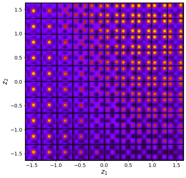
tvae_z_mean, tvae_z_sd = tvae.encode(train_data)
print('no. of defects', tvae_z_mean.shape)

z1 = tvae_z_mean[:, -2]
z2 = tvae_z_mean[:, -1]
tx = tvae_z_mean[:, -4]
ty = tvae_z_mean[:, -3]
no. of defects torch.Size([10917, 4])
Latent representation
# fig_tVAE_widget_1


combinations = [
    (z1, z2, r"$z_1$", r"$z_2$"),   # (b)
    (z1, tx, r"$z_1$", r"$t_x$"),   # (c)
    (z1, ty, r"$z_1$", r"$t_y$"),   # (d)
    (z2, tx, r"$z_2$", r"$t_x$"),   # (e)
    (z2, ty, r"$z_2$", r"$t_y$")    # (f)
]

# Create figure with 2 rows and 3 columns
fig, axes = plt.subplots(2, 3, figsize=(16, 10))
axes = axes.flatten()  # Flatten axes for easier looping

# (a) Latent manifold plot in the first position (dummy example here)
manifold = generate_latent_manifold(n=10, decoder=rvae.decode, target_size=(28, 28))

axes[0].imshow(manifold, cmap="gnuplot2", origin="upper", aspect="auto")
axes[0].set_xlabel(r"$z_1$", fontsize=16)
axes[0].set_ylabel(r"$z_2$", fontsize=16)
axes[0].set_xticks([]), axes[0].set_yticks([])
axes[0].text(-0.01, 1, 'a)', transform=axes[0].transAxes, fontsize=16, fontweight='bold', va='top', ha='right')

# Loop through combinations and plot KDE with scatter plots
for i, (x, y, xlabel, ylabel) in enumerate(combinations):
    ax = axes[i + 1]  # Start from the second subplot

    # KDE plot using seaborn
    sns.kdeplot(x=x, y=y, ax=ax, cmap="Oranges" ,levels=30, fill=True, alpha=0.6, thresh=0.005)

    # Scatter plot using seaborn
    sns.scatterplot(x=x, y=y, ax=ax, color="b", s=10, alpha=0.4, edgecolor="k")

    # Set labels, axis limits, and subplot labels
    ax.set_xlabel(xlabel, fontsize=16)
    ax.set_ylabel(ylabel, fontsize=16)
    ax.set_xticks([]), ax.set_yticks([])
    ax.text(-0.05, 1, f'{chr(98 + i)})', transform=ax.transAxes, fontsize=16, fontweight='bold', va='top', ha='right')

# Adjust layout for better spacing
plt.tight_layout()
plt.show()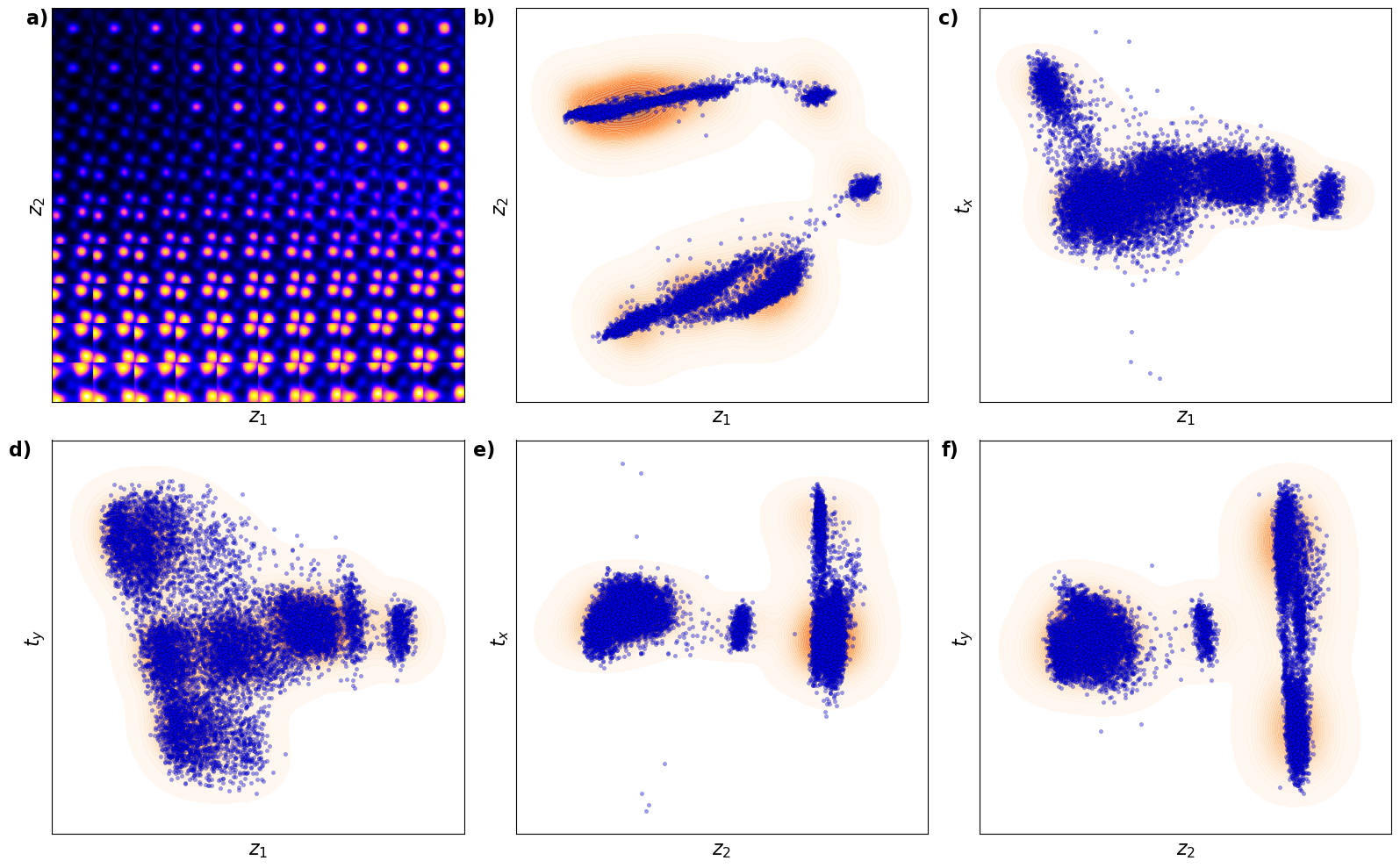
Now, th latent distribution start to look great. We see well defined clusters. It is tempting to say that these define the underpinning physics in the system.
# Static plotting of variables
def plot_all_variables():
    fig = plt.figure(figsize=(18, 12))

    # z1 plot
    ax1 = plt.subplot2grid((3, 3), (0, 0), colspan=1)
    scatter = ax1.scatter(coms_target[:, 1], coms_target[:, 0], c=z1, s=10, cmap='jet', marker="s")
    ax1.set_title("z1", fontsize=16, fontweight="bold")
    ax1.text(-0.1, 1.05, 'a)', transform=ax1.transAxes, fontsize=16, fontweight='bold', va='top', ha='right')
    ax1.axis("off")

    # z2 plot
    ax2 = plt.subplot2grid((3, 3), (0, 1), colspan=1)
    scatter = ax2.scatter(coms_target[:, 1], coms_target[:, 0], c=z2, s=10, cmap='jet', marker="s")
    ax2.set_title("z2", fontsize=16, fontweight="bold")
    ax2.text(-0.1, 1.05, 'b)', transform=ax2.transAxes, fontsize=16, fontweight='bold', va='top', ha='right')
    ax2.axis("off")

    # tx plot
    ax3 = plt.subplot2grid((3, 3), (0, 2), colspan=1)
    scatter = ax3.scatter(coms_target[:, 1], coms_target[:, 0], c=tx, s=10, cmap='jet', marker="s")
    ax3.set_title("tx", fontsize=16, fontweight="bold")
    ax3.text(-0.1, 1.05, 'c)', transform=ax3.transAxes, fontsize=16, fontweight='bold', va='top', ha='right')
    ax3.axis("off")

    # ty plot
    ax4 = plt.subplot2grid((3, 3), (1, 0), colspan=1)
    scatter = ax4.scatter(coms_target[:, 1], coms_target[:, 0], c=ty, s=10, cmap='jet', marker="s")
    ax4.set_title("ty", fontsize=16, fontweight="bold")
    ax4.text(-0.1, 1.05, 'd)', transform=ax4.transAxes, fontsize=16, fontweight='bold', va='top', ha='right')
    ax4.axis("off")

    # Px plot
    ax5 = plt.subplot2grid((3, 3), (1, 1), colspan=1)
    im = ax5.imshow(Px, cmap='jet', origin='lower')
    ax5.set_title("Ground Truth Px", fontsize=16, fontweight="bold")
    ax5.text(-0.1, 1.05, 'e)', transform=ax5.transAxes, fontsize=16, fontweight='bold', va='top', ha='right')
    ax5.axis("off")

    # Py plot
    ax6 = plt.subplot2grid((3, 3), (1, 2), colspan=1)
    im = ax6.imshow(Py, cmap='jet', origin='lower')
    ax6.set_title("Ground Truth Py", fontsize=16, fontweight="bold")
    ax6.text(-0.1, 1.05, 'f)', transform=ax6.transAxes, fontsize=16, fontweight='bold', va='top', ha='right')
    ax6.axis("off")

    plt.tight_layout()
    plt.show()
def plot_all_variables():
# Create a figure with a 2x3 grid of subplots
fig, axes = plt.subplots(2, 3, figsize=(18, 12))
# Plot z1
scatter = axes[0, 0].scatter(coms_target[:, 1], coms_target[:, 0], c=z1, s=10, cmap='jet', marker="s")
axes[0, 0].set_title("z1", fontsize=16, fontweight="bold")
axes[0, 0].text(-0.03, 1, 'a)', transform=axes[0, 0].transAxes, fontsize=16, fontweight='bold', va='top', ha='right')
axes[0, 0].axis("off")
# Plot z2
scatter = axes[0, 1].scatter(coms_target[:, 1], coms_target[:, 0], c=z2, s=10, cmap='jet', marker="s")
axes[0, 1].set_title("z2", fontsize=16, fontweight="bold")
axes[0, 1].text(-0.03, 1, 'b)', transform=axes[0, 1].transAxes, fontsize=16, fontweight='bold', va='top', ha='right')
axes[0, 1].axis("off")
# Plot tx
scatter = axes[0, 2].scatter(coms_target[:, 1], coms_target[:, 0], c=tx, s=10, cmap='jet', marker="s")
axes[0, 2].set_title("tx", fontsize=16, fontweight="bold")
axes[0, 2].text(-0.03, 1, 'c)', transform=axes[0, 2].transAxes, fontsize=16, fontweight='bold', va='top', ha='right')
axes[0, 2].axis("off")
# Plot ty
scatter = axes[1, 0].scatter(coms_target[:, 1], coms_target[:, 0], c=ty, s=10, cmap='jet', marker="s")
axes[1, 0].set_title("ty", fontsize=16, fontweight="bold")
axes[1, 0].text(-0.03, 1, 'd)', transform=axes[1, 0].transAxes, fontsize=16, fontweight='bold', va='top', ha='right')
axes[1, 0].axis("off")
# Plot Ground Truth Px
im = axes[1, 1].imshow(Px, cmap='jet', origin='lower')
axes[1, 1].set_title("Ground Truth Px", fontsize=16, fontweight="bold")
axes[1, 1].text(-0.03, 1, 'e)', transform=axes[1, 1].transAxes, fontsize=16, fontweight='bold', va='top', ha='right')
axes[1, 1].axis("off")
# Plot Ground Truth Py
im = axes[1, 2].imshow(Py, cmap='jet', origin='lower')
axes[1, 2].set_title("Ground Truth Py", fontsize=16, fontweight="bold")
axes[1, 2].text(-0.03, 1, 'f)', transform=axes[1, 2].transAxes, fontsize=16, fontweight='bold', va='top', ha='right')
axes[1, 2].axis("off")
# Adjust layout for better spacing
plt.tight_layout()
plt.show()# fig_tVAE_widget_2
plot_all_variables()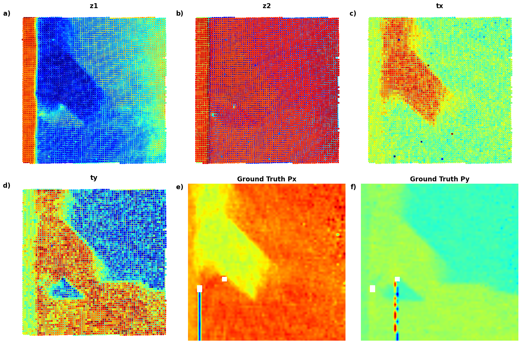
# import numpy as np
# import matplotlib.pyplot as plt
# from scipy.stats import gaussian_kde
# import ipywidgets as widgets
# from ipywidgets import interact

# # Define the data
# z1 = z1  # Latent variable 1
# z2 = z2  # Latent variable 2
# tx = tx  # Translation x
# ty = ty  # Translation y
# Px = SBFOdata[0]["ab_Px_resized"][main[0]:main[1], main[2]:main[3]]  # Ground truth Px
# Py = SBFOdata[0]["ab_Py_resized"][main[0]:main[1], main[2]:main[3]]  # Ground truth Py
# coms_target = coms_target  # Coordinates for scatter plots

# # Define options and data dictionary
# options = ["z1", "z2", "tx", "ty", "Ground Truth Px", "Ground Truth Py"]
# data_dict = {
#     "z1": z1,
#     "z2": z2,
#     "tx": tx,
#     "ty": ty,
#     "Ground Truth Px": Px,
#     "Ground Truth Py": Py
# }

# # Interactive function for plotting any two selected variables
# def interactive_plot(variable1, variable2):
#     fig, axes = plt.subplots(1, 2, figsize=(12, 6))

#     # Plot for variable 1
#     values1 = data_dict[variable1]
#     if variable1 in ["z1", "z2", "tx", "ty"]:
#         axes[0].scatter(coms_target[:, 1], coms_target[:, 0], c=values1, s=10, cmap='jet', marker="s")
#     else:
#         axes[0].imshow(values1, cmap='jet', origin='lower')
#     axes[0].set_title(variable1, fontsize=16)
#     axes[0].axis("off")

#     # Plot for variable 2
#     values2 = data_dict[variable2]
#     if variable2 in ["z1", "z2", "tx", "ty"]:
#         axes[1].scatter(coms_target[:, 1], coms_target[:, 0], c=values2, s=10, cmap='jet', marker="s")
#     else:
#         axes[1].imshow(values2, cmap='jet', origin='lower')
#     axes[1].set_title(variable2, fontsize=16)
#     axes[1].axis("off")

#     plt.tight_layout()
#     plt.show()
# ipywidgets.interact(
#     interactive_plot,
#     variable1=widgets.Dropdown(options=options, description="Variable 1"),
#     variable2=widgets.Dropdown(options=options, description="Variable 2"),
# );Now, the latent maps are becoming super interetsing as well. Note that translation vectors look almost exactly like polarization components. Note that the physics of ferroelectric is effectively shifft of the cntral atom vs. corner - so the translation representation reflects it. At the same time, z1 and z2 ahow chemical contrast and mistilt effects, with a bit of leackage of the poalrization informaiton.
trVAE
Now, let’s try all invariances - translation and rotation.
in_dim = (window_size[0],window_size[1])

# Initialize vanilla VAE
trvae = pv.models.iVAE(in_dim, latent_dim=2,   # Number of latent dimensions other than the invariancies
                     hidden_dim_e = [512, 512],
                     hidden_dim_d = [512, 512], # corresponds to the number of neurons in the hidden layers of the decoder
                     invariances=["r", "t"], seed=0)

# Initialize SVI trainer
trainer = pv.trainers.SVItrainer(trvae)

# Train for n epochs:
for e in range(10):
    trainer.step(train_loader)
    trainer.print_statistics()

trvae.save_weights('trvae_model')
print("Model saved successfully.")
Epoch: 1 Training loss: 766.7185
Epoch: 2 Training loss: 705.5259
Epoch: 3 Training loss: 693.5588
Epoch: 4 Training loss: 689.7197
Epoch: 5 Training loss: 686.3622
Epoch: 6 Training loss: 685.1326
Epoch: 7 Training loss: 684.1088
Epoch: 8 Training loss: 684.3674
Epoch: 9 Training loss: 683.2689
Epoch: 10 Training loss: 682.8993
Model saved successfully.
Varitional Auto Encoder manifold representation
trvae_laten_img = trvae.manifold2d(d=10, draw_grid = True, origin = 'lower')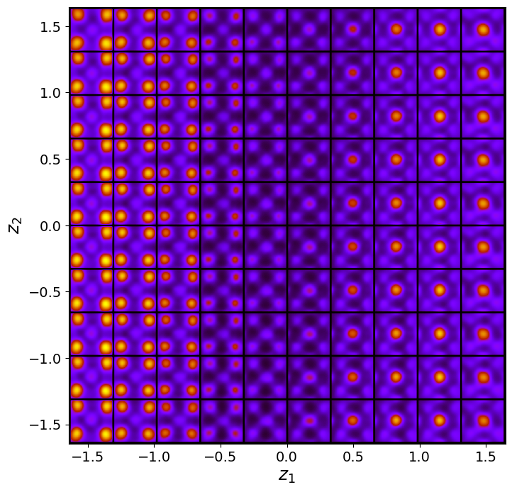
trvae_z_mean, trvae_z_sd = trvae.encode(train_data)
print('no. of defects', trvae_z_mean.shape)

z1 = trvae_z_mean[:, -2]
z2 = trvae_z_mean[:, -1]
ang = trvae_z_mean[:, 0]
tx = trvae_z_mean[:, -4]
ty = trvae_z_mean[:, -3]
no. of defects torch.Size([10917, 5])
Latent representation
# # fig_trVAE_widget_1

# z1_lim = [min(z1), max(z1)]
# z2_lim = [min(z2), max(z2)]
# ang_lim = [min(ang), max(ang)]
# tx_lim = [min(tx), max(tx)]
# ty_lim = [min(ty), max(ty)]

# # Define combinations for KDE scatter plots
# combinations = [
#     (z1, z2, r"$z_1$", r"$z_2$"),   # (b)
#     (z1, ang, r"$z_1$", r"$\theta$"),   # (c)
#     (z1, tx, r"$z_1$", r"$t_x$"),   # (d)
#     (z1, ty, r"$z_1$", r"$t_y$"),   # (e)
#     (z2, ang, r"$z_2$", r"$\theta$"),   # (f)
#     (z2, tx, r"$z_2$", r"$t_x$"),   # (g)
#     (z2, ty, r"$z_2$", r"$t_y$"),   # (h)
#     (ang, tx, r"$\theta$", r"$t_x$"),   # (i)
#     (ang, ty, r"$\theta$", r"$t_y$"),   # (j)
#     (tx, ty, r"$t_x$", r"$t_y$")    # (k)
# ]

# # Set up the figure with 4 rows and 3 columns
# fig, axes = plt.subplots(4, 3, figsize=(16, 16))
# axes = axes.flatten()  # Flatten axes for easy looping

# # (a) Latent manifold plot in the first position
# manifold = generate_latent_manifold(n=10, decoder=trvae.decode, target_size=(28, 28))
# axes[0].imshow(manifold, cmap="gnuplot2", origin="upper", aspect="auto")
# axes[0].set_xlabel(r"$z_1$", fontsize=16)
# axes[0].set_ylabel(r"$z_2$", fontsize=16)
# axes[0].set_xticks([]), axes[0].set_yticks([])
# axes[0].text(-0.1, 1.05, 'a)', transform=axes[0].transAxes, fontsize=16, fontweight='bold', va='top', ha='right')

# # Loop through combinations and plot KDE with scatter plots
# for i, (x, y, xlabel, ylabel) in enumerate(combinations):
#     ax = axes[i + 1]  # Start from the second subplot

#     # KDE plot
#     kde = gaussian_kde([x, y])
#     X, Y = np.meshgrid(np.linspace(min(x), max(x), 200), np.linspace(min(y), max(y), 200))
#     Z = kde(np.vstack([X.ravel(), Y.ravel()])).reshape(X.shape)
#     levels = np.linspace(Z.min() + 0.3 * (Z.max() - Z.min()), Z.max(), 30)
#     ax.contourf(X, Y, Z, levels=levels, cmap="jet", alpha=0.2)

#     # Scatter plot on top
#     ax.scatter(x, y, c="k", s=10, alpha=0.4, edgecolors="k")

#     # Set labels, axis limits, and subplot labels
#     ax.set_xlabel(xlabel, fontsize=16)
#     ax.set_ylabel(ylabel, fontsize=16)
#     ax.set_xlim(min(x), max(x)), ax.set_ylim(min(y), max(y))
#     ax.set_xticks([]), ax.set_yticks([])
#     ax.text(-0.02, 1, f'{chr(98 + i)})', transform=ax.transAxes, fontsize=16, fontweight='bold', va='top', ha='right')

# # Hide unused subplots to avoid empty maps
# for j in range(len(combinations) + 1, len(axes)):
#     axes[j].set_visible(False)

# # Adjust layout for better spacing
# plt.tight_layout()

# # Show the plot
# plt.show()
def plot_trVAE():
    # Set up the figure with 4 rows and 3 columns (11 maps + 1 for latent manifold)
    fig, axes = plt.subplots(4, 3, figsize=(18, 18))
    axes = axes.flatten()  # Flatten axes for easy looping

    # (a) Latent manifold plot in the first position
    manifold = generate_latent_manifold(n=10, decoder=trvae.decode, target_size=(28, 28))
    axes[0].imshow(manifold, cmap="gnuplot2", origin="upper", aspect="auto")
    axes[0].set_xlabel(r"$z_1$", fontsize=16)
    axes[0].set_ylabel(r"$z_2$", fontsize=16)
    axes[0].set_xticks([]), axes[0].set_yticks([])
    axes[0].text(-0.1, 1.05, 'a)', transform=axes[0].transAxes, fontsize=16, fontweight='bold', va='top', ha='right')

    # Define combinations for KDE scatter plots
    combinations = [
        (z1, z2, r"$z_1$", r"$z_2$"),   # (b)
        (z1, ang, r"$z_1$", r"$\theta$"),   # (c)
        (z1, tx, r"$z_1$", r"$t_x$"),   # (d)
        (z1, ty, r"$z_1$", r"$t_y$"),   # (e)
        (z2, ang, r"$z_2$", r"$\theta$"),   # (f)
        (z2, tx, r"$z_2$", r"$t_x$"),   # (g)
        (z2, ty, r"$z_2$", r"$t_y$"),   # (h)
        (ang, tx, r"$\theta$", r"$t_x$"),   # (i)
        (ang, ty, r"$\theta$", r"$t_y$"),   # (j)
        (tx, ty, r"$t_x$", r"$t_y$")    # (k)
    ]

    # Loop through combinations and plot KDE with scatter plots
    for i, (x, y, xlabel, ylabel) in enumerate(combinations):
        ax = axes[i + 1]  # Start from the second subplot

        # KDE plot using seaborn
        sns.kdeplot(x=x, y=y, ax=ax, cmap="Oranges", levels=30, fill=True, alpha=0.6, thresh=0.005)

        # Scatter plot on top using seaborn
        sns.scatterplot(x=x, y=y, ax=ax, color="b", s=10, alpha=0.4, edgecolor="k")

        # Set labels, axis limits, and subplot labels
        ax.set_xlabel(xlabel, fontsize=20, fontweight='bold')
        ax.set_ylabel(ylabel, fontsize=20, fontweight='bold')
        # ax.set_xlim(min(x), max(x)), ax.set_ylim(min(y), max(y))
        ax.set_xticks([]), ax.set_yticks([])
        ax.text(-0.05, 1, f'{chr(98 + i)})', transform=ax.transAxes, fontsize=20, fontweight='bold', va='top', ha='right')

    # Hide unused subplot (12th slot if no data)
    axes[len(combinations) + 1].axis("off")

    # Adjust layout for better spacing
    plt.tight_layout()

    # Show the plot
    plt.show()
# fig_trVAE_widget_1
plot_trVAE()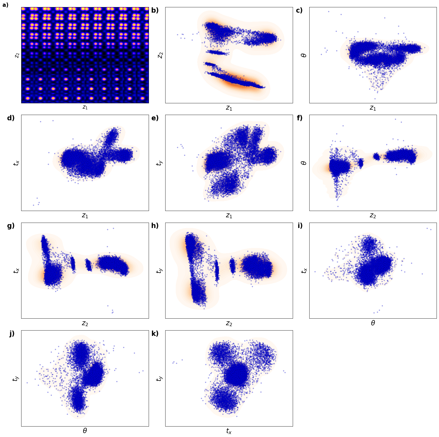
# combinations = [
#     (z1, z2, "z1", "z2"),
#     (z1, ang, "z1", "ang"),
#     (z1, tx, "z1", "tx"),
#     (z1, ty, "z1", "ty"),
#     (z2, ang, "z2", "ang"),
#     (z2, tx, "z2", "tx"),
#     (z2, ty, "z2", "ty"),
#     (ang, tx, "ang", "tx"),
#     (ang, ty, "ang", "ty"),
#     (tx, ty, "tx", "ty")
# ]

# # Set up the figure with 4 rows and 3 columns (enough to hold all combinations)
# fig, axes = plt.subplots(4, 3, figsize=(16, 16))

# # Flatten the axes array to loop through easily
# axes = axes.flatten()

# # Loop through combinations and plot them
# for i, (x, y, xlabel, ylabel) in enumerate(combinations):
#     sns.kdeplot(x=x, y=y, fill=True, ax=axes[i], cmap='Blues', alpha=0.4, levels=10)
#     axes[i].scatter(x, y, c="b", s=20, alpha=0.6, edgecolors="k")
#     axes[i].set_xlabel(xlabel, fontsize=18)
#     axes[i].set_ylabel(ylabel, fontsize=18)
#     axes[i].set_xticks([])
#     axes[i].set_yticks([])

# # Hide unused subplots to avoid empty maps
# for j in range(len(combinations), len(axes)):
#     axes[j].set_visible(False)

# # Adjust layout for better spacing
# plt.tight_layout()

# # Show the plot
# plt.show()
Kamyar, can you configure it it os it does not show empty maps?
Latent maps
# z1 = z1  # Latent variable 1
# z2 = z2  # Latent variable 2
# tx = tx  # Translation x
# ty = ty  # Translation y
# ang = ang  # Angular variable
# Px = SBFOdata[1]["ab_Px_resized"][main[0]:main[1], main[2]:main[3]]  # Ground truth Px
# Py = SBFOdata[1]["ab_Py_resized"][main[0]:main[1], main[2]:main[3]]  # Ground truth Py
# coms_target = coms_target  # Coordinates for scatter plots

# # Define options and data dictionary
# options = ["z1", "z2", "tx", "ty", "ang", "Ground Truth Px", "Ground Truth Py"]
# data_dict = {
#     "z1": z1,
#     "z2": z2,
#     "tx": tx,
#     "ty": ty,
#     "ang": ang,
#     "Ground Truth Px": Px,
#     "Ground Truth Py": Py
# }

# # Interactive function for plotting selected variables in a 3x3 grid
# def interactive_grid_plot(variable1, variable2):
#     # Data combinations to plot
#     data = [
#         (data_dict[variable1], variable1),
#         (data_dict[variable2], variable2)
#     ]

#     fig, axes = plt.subplots(1, 2, figsize=(12, 6))

#     # Plot for variable 1
#     values1, title1 = data[0]
#     if title1 in ["z1", "z2", "tx", "ty", "ang"]:
#         axes[0].scatter(coms_target[:, 1], coms_target[:, 0], c=values1, s=10, cmap="jet", marker="s")
#     else:
#         axes[0].imshow(values1, cmap="jet", origin="lower")
#     axes[0].set_title(title1, fontsize=16)
#     axes[0].axis("off")

#     # Plot for variable 2
#     values2, title2 = data[1]
#     if title2 in ["z1", "z2", "tx", "ty", "ang"]:
#         axes[1].scatter(coms_target[:, 1], coms_target[:, 0], c=values2, s=10, cmap="jet", marker="s")
#     else:
#         axes[1].imshow(values2, cmap="jet", origin="lower")
#     axes[1].set_title(title2, fontsize=16)
#     axes[1].axis("off")

#     plt.tight_layout()
#     plt.show()
# # fig_trVAE_widget_2
# ipywidgets.interact(
# interactive_grid_plot,
# variable1=widgets.Dropdown(options=options, value="z1", description="Variable 1"),
# variable2=widgets.Dropdown(options=options, value="z2", description="Variable 2")
# )<function __main__.interactive_grid_plot(variable1, variable2)>Px = SBFOdata[0]["ab_Px_resized"][main[0]:main[1], main[2]:main[3]] # Ground truth Px
Py = SBFOdata[0]["ab_Py_resized"][main[0]:main[1], main[2]:main[3]] # Ground truth Py
def plot_all_variables_in_grid():
fig, axes = plt.subplots(3, 3, figsize=(18, 18)) # 3x3 grid for all variables
axes = axes.flatten() # Flatten for easier indexing
# Define variables and titles
variables = [
(z1, r"$z_1$", 'a)'),
(z2, r"$z_2$", 'b)'),
(tx, r"$t_x$", 'c)'),
(ty, r"$t_y$", 'd)'),
(ang, r"$\theta$", 'e)'),
(Px, "Ground Truth Px", 'f)'),
(Py, "Ground Truth Py", 'g)')
]
# Loop over variables and plot
for i, (data, title, label) in enumerate(variables):
if title in [r"$z_1$", r"$z_2$", r"$t_x$", r"$t_y$", r"$\theta$"]: # Scatter plots
scatter = axes[i].scatter(coms_target[:, 1], coms_target[:, 0], c=data, s=10, cmap="jet", marker="s")
else: # Image plots
im = axes[i].imshow(data, cmap="jet", origin="lower")
axes[i].set_title(title, fontsize=20, fontweight="bold")
axes[i].text(-0.05, 1, label, transform=axes[i].transAxes, fontsize=20, fontweight="bold", va="top", ha="right")
axes[i].axis("off")
# Hide unused subplots (if any)
for j in range(len(variables), len(axes)):
axes[j].axis("off")
# Adjust layout
plt.tight_layout()
plt.show()
# fig_trVAE_widget_2


plot_all_variables_in_grid()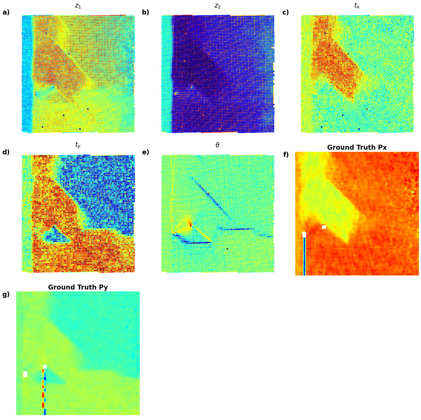
Bingo! Now our z2 map is only chemical and mistilt effects, tx and ty look like polarization, and angle is polarization rotation.
CVAE
However, our analysis above had a signnificant limitation. We were looking for latent representation common for A- and B-site cations, even though these are obviously different. Now, we are going to explore the conditional VAE, that consider cation type as known variable. Let’s see how it works!
condition 1: Set the conditiona as A and B site atoms of the material
w = (40,40)
min_sigma = 1
max_sigma = 5
threshold = 0.025
overlap = 0.0
descriptors_c, coms_target_c, all_atoms_c, coordinates_c, subimages_target_c = build_descriptor(w,
                                                                                                min_sigma,
                                                                                                max_sigma,
                                                                                                threshold,
                                                                                                overlap)

print(descriptors_c.shape)
print(subimages_target_c.shape)
print(coms_target_c.shape)
print(all_atoms_c.shape)
print(coordinates_c.shape)


labels_c, valid_subimages  = Fit_GMM(descriptors_c, 2, "full")
print(labels_c.shape)
(10917, 1600)
(10917, 40, 40)
(10917, 2)
(11813, 3)
(11813, 2)
(10917,)
plt.figure(figsize=(6, 6))
plt.imshow(image, cmap='gray')
plt.scatter(coms_target_c[:, 1], coms_target_c[:, 0], c=labels_c,  s=40, cmap='cool', marker= "o")


plt.xlim([400,700])
plt.ylim([400,700])
plt.axis('off')
plt.show()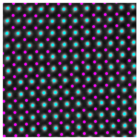
Data prepareation
subimages_target_reshaped = np.expand_dims(subimages_target, axis=-1)
train_data = torch.tensor(subimages_target_reshaped[:,:,:,0]).float()
lab_train = pv.utils.to_onehot(tt(labels_c).to(torch.int64), 2)
train_loader = pv.utils.init_dataloader(train_data.unsqueeze(1), lab_train, batch_size=48)
in_dim = (window_size[0],window_size[1])
# Initialize vanilla VAE
Cvae = pv.models.iVAE(in_dim, latent_dim=2, c_dim = 2, # Number of latent conditions
hidden_dim_e = [512, 512],
hidden_dim_d = [512, 512], # corresponds to the number of neurons in the hidden layers of the decoder
invariances=None, seed=0)
# Initialize SVI trainer
trainer = pv.trainers.SVItrainer(Cvae)
# Train for n epochs:
for e in range(10):
trainer.step(train_loader)
trainer.print_statistics()
Cvae.save_weights('cvae_model')
print("Model saved successfully.")Epoch: 1 Training loss: 693.8237
Epoch: 2 Training loss: 677.4711
Epoch: 3 Training loss: 676.1651
Epoch: 4 Training loss: 675.5241
Epoch: 5 Training loss: 675.1202
Epoch: 6 Training loss: 674.9503
Epoch: 7 Training loss: 674.7996
Epoch: 8 Training loss: 674.5394
Epoch: 9 Training loss: 674.6851
Epoch: 10 Training loss: 674.2635
Model saved successfully.
Varitional Auto Encoder manifold representation
def generate_latent_manifold_C(n=10, decoder=None, target_size=(28, 28), condition=None):
    """
    Generate a conditional latent manifold grid over the entire latent space.
    """
    # Define grid bounds across latent space
    grid_x = np.linspace(min(z1), max(z1), n)
    grid_y = np.linspace(min(z2), max(z2), n)

    # Dynamically infer output shape
    latent_sample = torch.tensor([[grid_x[0], grid_y[0]]], dtype=torch.float32)
    if condition is not None:
        condition = condition.view(1, -1)  # Ensure condition is 2D with shape (1, num_classes)
        latent_sample = torch.cat((latent_sample, condition), dim=1)

    with torch.no_grad():
        X_decoded = decoder(latent_sample)
    decoded_shape = X_decoded.shape[-2:] if len(X_decoded.shape) > 2 else (X_decoded.shape[-1], X_decoded.shape[-1])

    # Initialize the manifold grid
    height, width = target_size
    manifold = np.zeros((height * n, width * n))

    # Generate conditional manifold
    for i, yi in enumerate(grid_x):
        for j, xi in enumerate(grid_y):
            latent_sample = torch.tensor([[xi, yi]], dtype=torch.float32)
            if condition is not None:
                latent_sample = torch.cat((latent_sample, condition), dim=1)  # Concatenate condition
            with torch.no_grad():
                X_decoded = decoder(latent_sample).reshape(decoded_shape)
            resized_image = zoom(X_decoded, zoom=(height / X_decoded.shape[-2], width / X_decoded.shape[-1]))
            manifold[i * height: (i + 1) * height, j * width: (j + 1) * width] = resized_image

    return manifold
n_classes = 2 # Number of conditions
from torch.nn.functional import one_hot
for cls in range(n_classes):
condition = torch.tensor([[cls]], dtype=torch.int64) # Class as integer
condition_onehot = one_hot(condition, num_classes=n_classes).float() # One-hot encode
# Generate and display manifold for each class
manifold = generate_latent_manifold_C(n=10, decoder=Cvae.decode, target_size=(28, 28), condition=condition_onehot)
plt.figure(figsize=(6, 6))
plt.imshow(manifold, cmap="gnuplot2", origin="upper")
plt.title(f"Conditional Latent Manifold for Class {cls}")
plt.axis("off")
plt.show()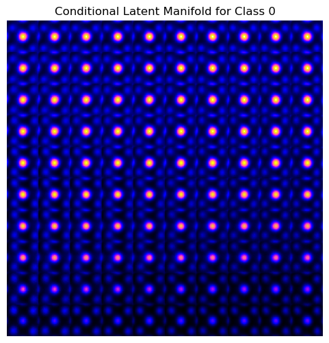
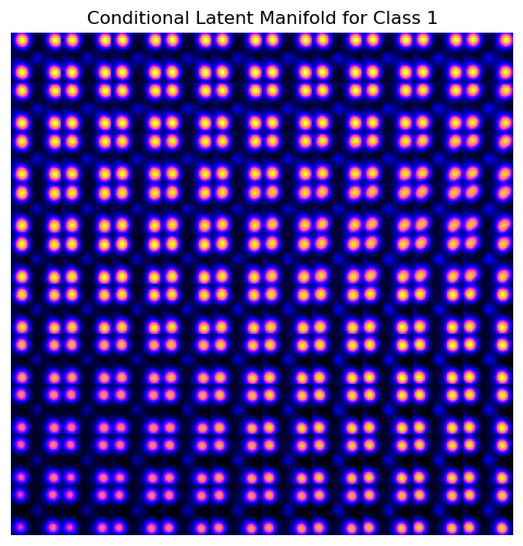
# for cls in range(2):
#     cls = pv.utils.to_onehot(tt([cls,]), 2)
#     Cvae.manifold2d(d=10, y=cls, cmap="gnuplot")
Cvae_z_mean, Cvae_z_sd = Cvae.encode(train_data.unsqueeze(-1), lab_train)
print('no. of defects', Cvae_z_mean.shape)
z1 = Cvae_z_mean[:, -2]
z2 = Cvae_z_mean[:, -1]no. of defects torch.Size([10917, 2])
import matplotlib.pyplot as plt
from scipy.stats import gaussian_kde
import numpy as np
import torch
from torch.nn.functional import one_hot
from scipy.ndimage import zoomdef generate_latent_manifold_C(n=10, decoder=None, target_size=(28, 28), condition=None):
# Define grid bounds across latent space
grid_x = np.linspace(min(z1), max(z1), n)
grid_y = np.linspace(min(z2), max(z2), n)
# Dynamically infer output shape
latent_sample = torch.tensor([[grid_x[0], grid_y[0]]], dtype=torch.float32)
if condition is not None:
latent_sample = torch.cat((latent_sample, condition), dim=1)
with torch.no_grad():
X_decoded = decoder(latent_sample)
# Check output dimensions
if len(X_decoded.shape) == 1:
X_decoded = X_decoded.reshape(1, -1) # Flattened output
output_size = X_decoded.shape[-1] if len(X_decoded.shape) == 2 else X_decoded.shape[-2:]
# Initialize the manifold
height, width = target_size
manifold = np.zeros((height * n, width * n))
# Generate the manifold grid
for i, yi in enumerate(grid_x):
for j, xi in enumerate(grid_y):
latent_sample = torch.tensor([[xi, yi]], dtype=torch.float32)
if condition is not None:
latent_sample = torch.cat((latent_sample, condition), dim=1)
with torch.no_grad():
X_decoded = decoder(latent_sample)
if len(X_decoded.shape) == 1:
X_decoded = X_decoded.reshape(1, -1) # Handle flattened output
resized_image = zoom(X_decoded.numpy().reshape(output_size),
zoom=(height / output_size[0], width / output_size[1]))
manifold[i * height: (i + 1) * height, j * width: (j + 1) * width] = resized_image
return manifold
# condition_0 = torch.nn.functional.one_hot(torch.tensor([0]), num_classes=2).float()
# manifold_0 = generate_latent_manifold_C(n=10, decoder=Cvae.decode, target_size=(28, 28), condition=condition_0)
# condition_1 = torch.nn.functional.one_hot(torch.tensor([1]), num_classes=2).float()
# manifold_1 = generate_latent_manifold_C(n=10, decoder=Cvae.decode, target_size=(28, 28), condition=condition_1)
# # KDE for z1 vs z2
# kde = gaussian_kde([z1, z2])
# X, Y = np.meshgrid(np.linspace(min(z1), max(z1), 200), np.linspace(min(z2), max(z2), 200))
# Z = kde(np.vstack([X.ravel(), Y.ravel()])).reshape(X.shape)
# levels = np.linspace(Z.min() + 0.2 * (Z.max() - Z.min()), Z.max(), 30)
# # Create the figure with 1 row and 3 columns
# fig, axes = plt.subplots(1, 3, figsize=(18, 6))
# # (a) Latent manifold for class 0
# axes[0].imshow(manifold_0, cmap="gnuplot2", origin="upper", aspect="auto")
# # axes[0].set_title("Manifold for Class 0", fontsize=16)
# axes[0].set_xlabel(r"$z_1$", fontsize=14)
# axes[0].set_ylabel(r"$z_2$", fontsize=14)
# axes[0].set_xticks([]), axes[0].set_yticks([])
# # (b) Latent manifold for class 1
# axes[1].imshow(manifold_1, cmap="gnuplot2", origin="upper", aspect="auto")
# # axes[1].set_title("Manifold for Class 1", fontsize=16)
# axes[1].set_xlabel(r"$z_1$", fontsize=14)
# axes[1].set_ylabel(r"$z_2$", fontsize=14)
# axes[1].set_xticks([]), axes[1].set_yticks([])
# # (c) Scatter plot of z1 vs z2 with KDE contours
# axes[2].scatter(z1, z2, c=labels_c, s=20, cmap="jet", edgecolors="k", alpha=0.7)
# axes[2].contourf(X, Y, Z, levels=levels, cmap="jet", alpha=0.2) # Add KDE contours
# axes[2].set_xlabel(r"$z_1$", fontsize=14)
# axes[2].set_ylabel(r"$z_2$", fontsize=14)
# axes[2].set_xticks([]), axes[2].set_yticks([])
# # Adjust layout and display
# plt.tight_layout()
# plt.show()def plot_CVAE():
# Set up the figure with 1 row and 3 columns
fig, axes = plt.subplots(1, 3, figsize=(18, 6))
# (a) Latent manifold for class 0
condition_0 = torch.nn.functional.one_hot(torch.tensor([0]), num_classes=2).float()
manifold_0 = generate_latent_manifold_C(n=10, decoder=Cvae.decode, target_size=(28, 28), condition=condition_0)
axes[0].imshow(manifold_0, cmap="gnuplot2", origin="upper", aspect="auto")
axes[0].set_xlabel(r"$z_1$", fontsize=20)
axes[0].set_ylabel(r"$z_2$", fontsize=20)
axes[0].set_xticks([]), axes[0].set_yticks([])
axes[0].text(-0.05, 1, 'a)', transform=axes[0].transAxes, fontsize=20, fontweight='bold', va='top', ha='right')
# (b) Latent manifold for class 1
condition_1 = torch.nn.functional.one_hot(torch.tensor([1]), num_classes=2).float()
manifold_1 = generate_latent_manifold_C(n=10, decoder=Cvae.decode, target_size=(28, 28), condition=condition_1)
axes[1].imshow(manifold_1, cmap="gnuplot2", origin="upper", aspect="auto")
axes[1].set_xlabel(r"$z_1$", fontsize=20, fontweight='bold')
axes[1].set_ylabel(r"$z_2$", fontsize=20, fontweight='bold')
axes[1].set_xticks([]), axes[1].set_yticks([])
axes[1].text(-0.05, 1, 'b)', transform=axes[1].transAxes, fontsize=20, fontweight='bold', va='top', ha='right')
# (c) Scatter plot of z1 vs z2 with KDE using sns
sns.kdeplot(x=z1, y=z2, ax=axes[2], cmap="Oranges", levels=60, fill=True, alpha=0.7, thresh=0.005)
sns.scatterplot(x=z1, y=z2, ax=axes[2], hue=labels_c, palette="coolwarm", s=20, edgecolor="k", alpha=0.7, legend=False)
axes[2].set_xlabel(r"$z_1$", fontsize=20, fontweight='bold')
axes[2].set_ylabel(r"$z_2$", fontsize=20, fontweight='bold')
axes[2].set_xticks([]), axes[2].set_yticks([])
axes[2].text(-0.05, 1, 'c)', transform=axes[2].transAxes, fontsize=20, fontweight='bold', va='top', ha='right')
# Adjust layout for better spacing
plt.tight_layout()
plt.show()
# fig_CVAE_widget_1
plot_CVAE()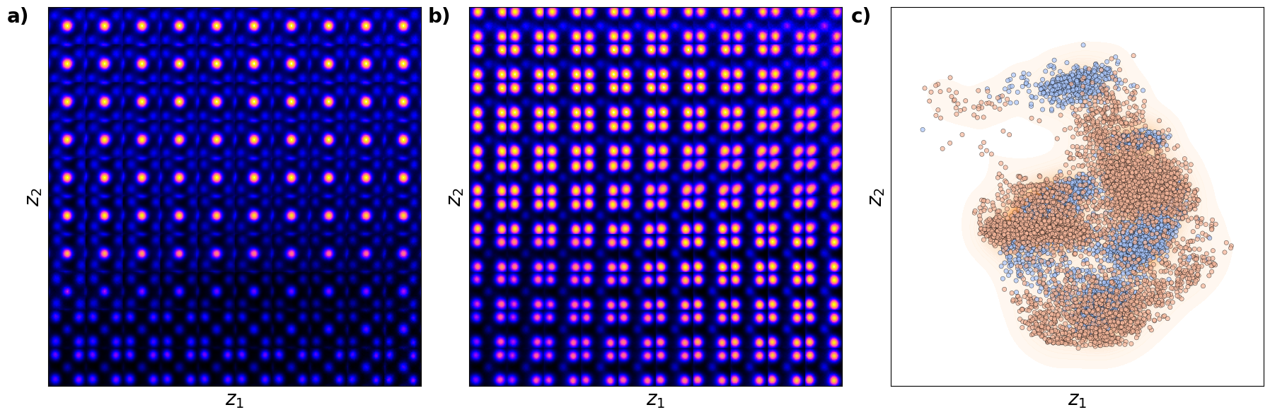
Now we have two latent spaces - for A-type and B-type separately.
Cvae_z_mean, Cvae_z_sd = Cvae.encode(train_data.unsqueeze(-1), lab_train)
print('no. of defects', Cvae_z_mean.shape)

z1 = Cvae_z_mean[:, -2]
z2 = Cvae_z_mean[:, -1]
no. of defects torch.Size([10917, 2])
Latent representation
# plt.figure(figsize=(6, 6))

# # Create the KDE plot for density estimation
# sns.kdeplot(x=z1, y=z2, cmap='Spectral', fill=True, alpha=0.3, levels=10)

# # Create the scatter plot with enhancements
# plt.scatter(z1, z2, c=labels_c, s=20, alpha=0.7, edgecolors="k", cmap='jet')

# # Set labels and remove ticks for a minimalist style
# plt.xlabel("z1", fontsize=20)
# plt.ylabel("z2", fontsize=20)
# plt.xticks([])
# plt.yticks([])

# # Show the plot
# plt.show()
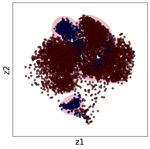
Latent maps
import numpy as np
import matplotlib.pyplot as plt
import ipywidgets as widgets
from ipywidgets import interact

# Define the data
z1 = z1  # Latent variable 1
z2 = z2  # Latent variable 2
Px = SBFOdata[0]["ab_Px_resized"][main[0]:main[1], main[2]:main[3]]  # Ground Truth Px
Py = SBFOdata[0]["ab_Py_resized"][main[0]:main[1], main[2]:main[3]]  # Ground Truth Py
coms_target = coms_target  # Coordinates for scatter plots

# Define options and data dictionary
options = ["z1", "z2", "Ground Truth Px", "Ground Truth Py"]
data_dict = {
    "z1": z1,
    "z2": z2,
    "Ground Truth Px": Px,
    "Ground Truth Py": Py
}

# Interactive function for plotting any two selected variables
def interactive_plot(variable1, variable2):
    """
    Display two variables side-by-side interactively as scatter plots or images.
    """
    fig, axes = plt.subplots(1, 2, figsize=(12, 6))

    # Plot for variable 1
    values1 = data_dict[variable1]
    if variable1 in ["z1", "z2"]:
        axes[0].scatter(coms_target[:, 1], coms_target[:, 0], c=values1, s=10, cmap='jet', marker="s")
    else:
        axes[0].imshow(values1, cmap='jet', origin='lower')
    axes[0].set_title(variable1, fontsize=16)
    axes[0].axis("off")

    # Plot for variable 2
    values2 = data_dict[variable2]
    if variable2 in ["z1", "z2"]:
        axes[1].scatter(coms_target[:, 1], coms_target[:, 0], c=values2, s=10, cmap='jet', marker="s")
    else:
        axes[1].imshow(values2, cmap='jet', origin='lower')
    axes[1].set_title(variable2, fontsize=16)
    axes[1].axis("off")

    plt.tight_layout()
    plt.show()
# ipywidgets.interact(
#     interactive_plot,
#     variable1=widgets.Dropdown(options=options, description="Variable 1", value="z1"),
#     variable2=widgets.Dropdown(options=options, description="Variable 2", value="z2")
# )<function __main__.interactive_plot(variable1, variable2)>def plot_all_maps():
fig, axes = plt.subplots(2, 2, figsize=(12, 12))
# (a) z1 map
scatter = axes[0, 0].scatter(coms_target[:, 1], coms_target[:, 0], c=z1, s=10, cmap='jet', marker="s")
axes[0, 0].set_title("z1", fontsize=16, fontweight="bold")
axes[0, 0].text(-0.05, 1, 'a)', transform=axes[0, 0].transAxes, fontsize=16, fontweight='bold', va='top', ha='right')
axes[0, 0].axis("off")
# (b) z2 map
scatter = axes[0, 1].scatter(coms_target[:, 1], coms_target[:, 0], c=z2, s=10, cmap='jet', marker="s")
axes[0, 1].set_title("z2", fontsize=16, fontweight="bold")
axes[0, 1].text(-0.05, 1, 'b)', transform=axes[0, 1].transAxes, fontsize=16, fontweight='bold', va='top', ha='right')
axes[0, 1].axis("off")
# (c) Ground Truth Px map
im = axes[1, 0].imshow(Px, cmap='jet', origin='lower')
axes[1, 0].set_title("Ground Truth Px", fontsize=16, fontweight="bold")
axes[1, 0].text(-0.05, 1, 'c)', transform=axes[1, 0].transAxes, fontsize=16, fontweight='bold', va='top', ha='right')
axes[1, 0].axis("off")
# (d) Ground Truth Py map
im = axes[1, 1].imshow(Py, cmap='jet', origin='lower')
axes[1, 1].set_title("Ground Truth Py", fontsize=16, fontweight="bold")
axes[1, 1].text(-0.05, 1, 'd)', transform=axes[1, 1].transAxes, fontsize=16, fontweight='bold', va='top', ha='right')
axes[1, 1].axis("off")
# Adjust layout and show
plt.tight_layout()
plt.show()
# fig_CVAE_widget_2


plot_all_maps()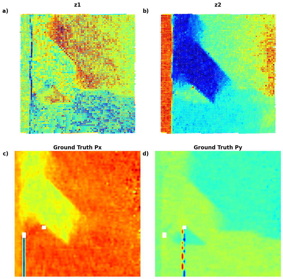
Now, we are starting to see something new. Note that we see anomalous behavior of the z1 at the “diffuse” domain walls. So, what’s going on? Lets start to add invariances!
CrVAE
in_dim = (window_size[0],window_size[1])

# Initialize vanilla VAE
Crvae = pv.models.iVAE(in_dim, latent_dim=2, c_dim = 2, # Number of latent conditions
                     hidden_dim_e = [512,512],   # corresponds to the number of neurons in the hidden layers of the encoder
                     hidden_dim_d = [512,512],# corresponds to the number of neurons in the hidden layers of the decoder
                       # corresponds to the number of neurons in the hidden layers of the decoder
                     invariances=["r"], seed=0)
# Initialize SVI trainer
trainer = pv.trainers.SVItrainer(Crvae)

# Train for n epochs:
for e in range(10):
    trainer.step(train_loader)
    trainer.print_statistics()

Crvae.save_weights('crvae_model')
print("Model saved successfully.")
---------------------------------------------------------------------------
KeyboardInterrupt Traceback (most recent call last)
Cell In[24], line 14
12 # Train for n epochs:
13 for e in range(10):
---> 14 trainer.step(train_loader)
15 trainer.print_statistics()
17 Crvae.save_weights('crvae_model')
File ~/miniconda3/envs/ferro_VAE/lib/python3.12/site-packages/pyroved/trainers/svi.py:157, in SVItrainer.step(self, train_loader, test_loader, **kwargs)
139 def step(self,
140 train_loader: Type[torch.utils.data.DataLoader],
141 test_loader: Optional[Type[torch.utils.data.DataLoader]] = None,
142 **kwargs: float) -> None:
143 """
144 Single training and (optionally) evaluation step
145
(...)
155 Default value is 1 (i.e. no scaling)
156 """
--> 157 train_loss = self.train(train_loader, **kwargs)
158 self.loss_history["training_loss"].append(train_loss)
159 if test_loader is not None:
File ~/miniconda3/envs/ferro_VAE/lib/python3.12/site-packages/pyroved/trainers/svi.py:110, in SVItrainer.train(self, train_loader, **kwargs)
108 else: # VED or cVAE mode
109 x, y = data
--> 110 loss = self.svi.step(
111 x.to(self.device), y.to(self.device), **kwargs)
112 # do ELBO gradient and accumulate loss
113 epoch_loss += loss
File ~/miniconda3/envs/ferro_VAE/lib/python3.12/site-packages/pyro/infer/svi.py:145, in SVI.step(self, *args, **kwargs)
143 # get loss and compute gradients
144 with poutine.trace(param_only=True) as param_capture:
--> 145 loss = self.loss_and_grads(self.model, self.guide, *args, **kwargs)
147 params = set(
148 site["value"].unconstrained() for site in param_capture.trace.nodes.values()
149 )
151 # actually perform gradient steps
152 # torch.optim objects gets instantiated for any params that haven't been seen yet
File ~/miniconda3/envs/ferro_VAE/lib/python3.12/site-packages/pyro/infer/trace_elbo.py:157, in Trace_ELBO.loss_and_grads(self, model, guide, *args, **kwargs)
153 if trainable_params and getattr(
154 surrogate_loss_particle, "requires_grad", False
155 ):
156 surrogate_loss_particle = surrogate_loss_particle / self.num_particles
--> 157 surrogate_loss_particle.backward(retain_graph=self.retain_graph)
158 warn_if_nan(loss, "loss")
159 return loss
File ~/miniconda3/envs/ferro_VAE/lib/python3.12/site-packages/torch/_tensor.py:581, in Tensor.backward(self, gradient, retain_graph, create_graph, inputs)
571 if has_torch_function_unary(self):
572 return handle_torch_function(
573 Tensor.backward,
574 (self,),
(...)
579 inputs=inputs,
580 )
--> 581 torch.autograd.backward(
582 self, gradient, retain_graph, create_graph, inputs=inputs
583 )
File ~/miniconda3/envs/ferro_VAE/lib/python3.12/site-packages/torch/autograd/__init__.py:347, in backward(tensors, grad_tensors, retain_graph, create_graph, grad_variables, inputs)
342 retain_graph = create_graph
344 # The reason we repeat the same comment below is that
345 # some Python versions print out the first line of a multi-line function
346 # calls in the traceback and some print out the last line
--> 347 _engine_run_backward(
348 tensors,
349 grad_tensors_,
350 retain_graph,
351 create_graph,
352 inputs,
353 allow_unreachable=True,
354 accumulate_grad=True,
355 )
File ~/miniconda3/envs/ferro_VAE/lib/python3.12/site-packages/torch/autograd/graph.py:825, in _engine_run_backward(t_outputs, *args, **kwargs)
823 unregister_hooks = _register_logging_hooks_on_whole_graph(t_outputs)
824 try:
--> 825 return Variable._execution_engine.run_backward( # Calls into the C++ engine to run the backward pass
826 t_outputs, *args, **kwargs
827 ) # Calls into the C++ engine to run the backward pass
828 finally:
829 if attach_logging_hooks:
KeyboardInterrupt: Varitional Auto Encoder manifold representation
for cls in range(2):
    cls = pv.utils.to_onehot(tt([cls,]), 2)
    Crvae.manifold2d(d=10, y=cls, cmap="gnuplot")
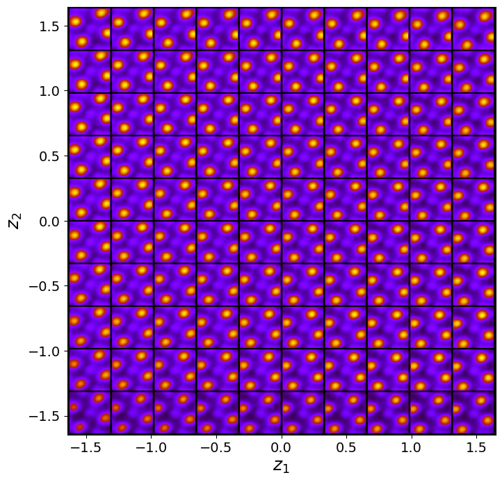
Crvae_z_mean, Crvae_z_sd = Crvae.encode(train_data.unsqueeze(-1), lab_train)
print('no. of defects', Crvae_z_mean.shape)

z1 = Crvae_z_mean[:, -2]
z2 = Crvae_z_mean[:, -1]
ang = Crvae_z_mean[:, 0]
no. of defects torch.Size([10917, 3])
Latent representation
def plot_CrVAE():
    # Set up the figure with 2 rows and 3 columns
    fig, axes = plt.subplots(2, 3, figsize=(18, 12))

    # (a) Latent manifold for class 0
    condition_0 = torch.nn.functional.one_hot(torch.tensor([0]), num_classes=2).float()
    manifold_0 = generate_latent_manifold_C(n=10, decoder=Cvae.decode, target_size=(28, 28), condition=condition_0)
    axes[0, 0].imshow(manifold_0, cmap="gnuplot2", origin="upper", aspect="auto")
    axes[0, 0].set_xlabel(r"$z_1$", fontsize=20, fontweight="bold")
    axes[0, 0].set_ylabel(r"$z_2$", fontsize=20, fontweight="bold")
    axes[0, 0].set_xticks([]), axes[0, 0].set_yticks([])
    axes[0, 0].text(-0.05, 1, 'a)', transform=axes[0, 0].transAxes, fontsize=20, fontweight='bold', va='top', ha='right')

    # (b) Latent manifold for class 1
    condition_1 = torch.nn.functional.one_hot(torch.tensor([1]), num_classes=2).float()
    manifold_1 = generate_latent_manifold_C(n=10, decoder=Cvae.decode, target_size=(28, 28), condition=condition_1)
    axes[0, 1].imshow(manifold_1, cmap="gnuplot2", origin="upper", aspect="auto")
    axes[0, 1].set_xlabel(r"$z_1$", fontsize=20, fontweight="bold")
    axes[0, 1].set_ylabel(r"$z_2$", fontsize=20, fontweight="bold")
    axes[0, 1].set_xticks([]), axes[0, 1].set_yticks([])
    axes[0, 1].text(-0.05, 1, 'b)', transform=axes[0, 1].transAxes, fontsize=20, fontweight='bold', va='top', ha='right')

    # (c) KDE and scatter plot of z1 vs z2
    sns.kdeplot(x=z1, y=z2, ax=axes[0, 2], cmap="Oranges", levels=30, fill=True, alpha=0.6, thresh=0.005)
    sns.scatterplot(x=z1, y=z2, ax=axes[0, 2], hue=labels_c, palette="coolwarm", s=20, edgecolor="k", alpha=0.7, legend=False)
    axes[0, 2].set_xlabel(r"$z_1$", fontsize=20, fontweight="bold")
    axes[0, 2].set_ylabel(r"$z_2$", fontsize=20, fontweight="bold")
    axes[0, 2].set_xticks([]), axes[0, 2].set_yticks([])
    axes[0, 2].text(-0.05, 1, 'c)', transform=axes[0, 2].transAxes, fontsize=20, fontweight='bold', va='top', ha='right')

    # (d) KDE and scatter plot of angle vs z1
    sns.kdeplot(x=ang, y=z1, ax=axes[1, 0], cmap="Oranges", levels=30, fill=True, alpha=0.6, thresh=0.005)
    sns.scatterplot(x=ang, y=z1, ax=axes[1, 0], hue=labels_c, palette="coolwarm", s=20, edgecolor="k", alpha=0.7, legend=False)
    axes[1, 0].set_xlabel(r"$\theta$", fontsize=20, fontweight="bold")
    axes[1, 0].set_ylabel(r"$z_1$", fontsize=20, fontweight="bold")
    axes[1, 0].set_xticks([]), axes[1, 0].set_yticks([])
    axes[1, 0].text(-0.05, 1, 'd)', transform=axes[1, 0].transAxes, fontsize=20, fontweight='bold', va='top', ha='right')

    # (e) KDE and scatter plot of angle vs z2
    sns.kdeplot(x=ang, y=z2, ax=axes[1, 1], cmap="Oranges", levels=30, fill=True, alpha=0.6, thresh=0.005)
    sns.scatterplot(x=ang, y=z2, ax=axes[1, 1], hue=labels_c, palette="coolwarm", s=20, edgecolor="k", alpha=0.7, legend=False)
    axes[1, 1].set_xlabel(r"$\theta$", fontsize=20, fontweight="bold")
    axes[1, 1].set_ylabel(r"$z_2$", fontsize=20, fontweight="bold")
    axes[1, 1].set_xticks([]), axes[1, 1].set_yticks([])
    axes[1, 1].text(-0.05, 1, 'e)', transform=axes[1, 1].transAxes, fontsize=20, fontweight='bold', va='top', ha='right')

    # (f) KDE and scatter plot of z1 vs z2 with angle as hue
    sns.kdeplot(x=z1, y=z2, ax=axes[1, 2], cmap="Oranges", levels=30, fill=True, alpha=0.6, thresh=0.005)
    sns.scatterplot(x=z1, y=z2, ax=axes[1, 2], hue=ang, palette="coolwarm", s=20, edgecolor="k", alpha=0.7, legend=False)
    axes[1, 2].set_xlabel(r"$z_1$", fontsize=20, fontweight="bold")
    axes[1, 2].set_ylabel(r"$z_2$", fontsize=20, fontweight="bold")
    axes[1, 2].set_xticks([]), axes[1, 2].set_yticks([])
    axes[1, 2].text(-0.05, 1, 'f)', transform=axes[1, 2].transAxes, fontsize=20, fontweight='bold', va='top', ha='right')

    # Adjust layout for better spacing
    plt.tight_layout()

    # Display the plot
    plt.show()
# fig_CrVAE_widget_1

plot_CrVAE()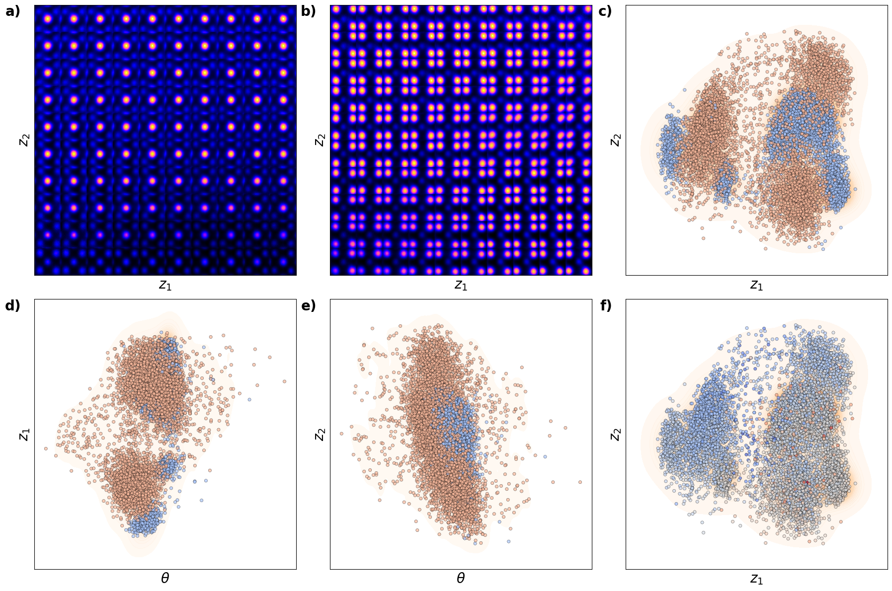
Latent maps
def plot_variables():
    # Define the data to plot
    data = [
        (z1, "z1"),
        (z2, "z2"),
        (ang, "ang"),
        (SBFOdata[0]["ab_Px_resized"][main[0]:main[1], main[2]:main[3]], "Ground Truth Px"),
        (SBFOdata[0]["ab_Py_resized"][main[0]:main[1], main[2]:main[3]], "Ground Truth Py")
    ]

    # Create figure with 2 rows and 3 columns
    fig, axes = plt.subplots(2, 3, figsize=(16, 10))
    axes = axes.flatten()  # Flatten axes for easier looping

    # Loop through the data and plot
    for i, (values, title) in enumerate(data):
        if i < 3:  # Scatter plot for z1, z2, and ang
            scatter = axes[i].scatter(coms_target[:, 1], coms_target[:, 0], c=values, s=10, cmap='jet', marker="s")
        else:  # Imshow for Ground Truth Px and Py
            im = axes[i].imshow(values, cmap='jet', origin='lower')

        # Add title and axis labels
        axes[i].set_title(title, fontsize=18, fontweight="bold")
        axes[i].axis("off")
        axes[i].text(-0.05, 1, f'{chr(97 + i)})', transform=axes[i].transAxes, fontsize=18, fontweight='bold', va='top', ha='right')

    # Hide the last subplot if unused
    axes[-1].set_visible(False)

    # Adjust layout for better spacing
    plt.tight_layout()

    # Display the plot
    plt.show()
# fig_CrVAE_widget_2
plot_variables()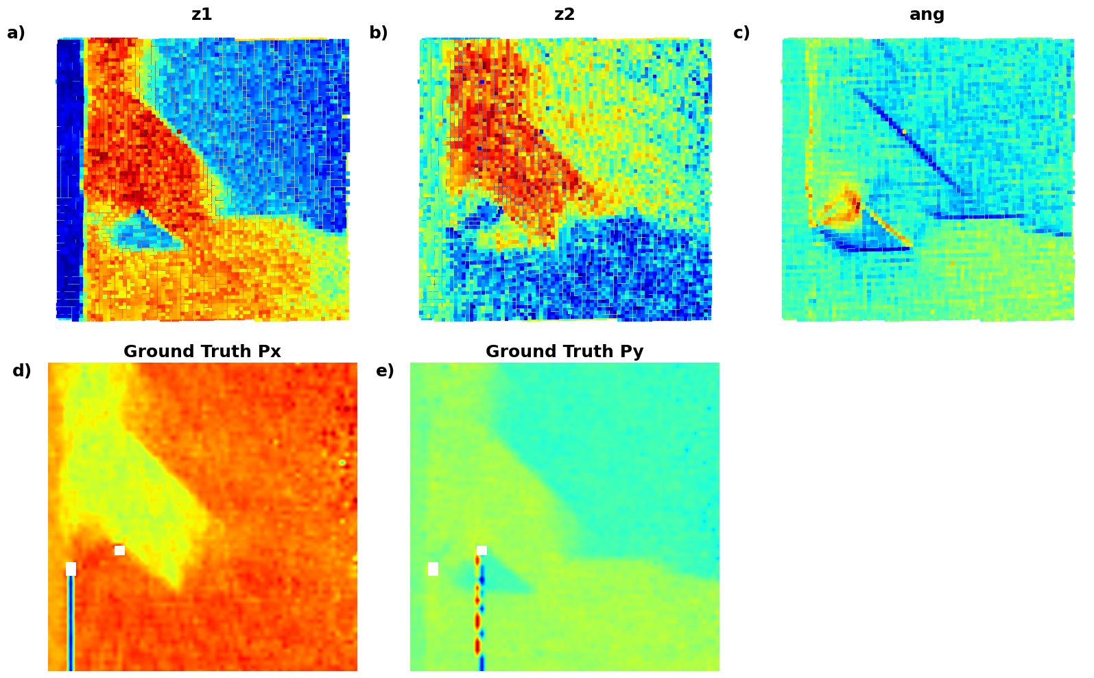
CtVAE
in_dim = (window_size[0],window_size[1])

# Initialize vanilla VAE
Ctvae = pv.models.iVAE(in_dim, latent_dim=2, c_dim = 2, # Number of latent conditions
                     hidden_dim_e = [512,512],   # corresponds to the number of neurons in the hidden layers of the encoder
                     hidden_dim_d = [512,512],# corresponds to the number of neurons in the hidden layers of the decoder
                       # corresponds to the number of neurons in the hidden layers of the decoder
                     invariances=["t"], seed=0)
# Initialize SVI trainer
trainer = pv.trainers.SVItrainer(Ctvae)

# Train for n epochs:
for e in range(10):
    trainer.step(train_loader)
    trainer.print_statistics()

Ctvae.save_weights('ctvae_model')
print("Model saved successfully.")
Epoch: 1 Training loss: 770.1249
Epoch: 2 Training loss: 702.0833
Epoch: 3 Training loss: 687.3292
Epoch: 4 Training loss: 681.7201
Epoch: 5 Training loss: 679.9082
Epoch: 6 Training loss: 679.0873
Epoch: 7 Training loss: 678.3367
Epoch: 8 Training loss: 677.8529
Epoch: 9 Training loss: 678.0812
Epoch: 10 Training loss: 677.9746
Varitional Auto Encoder manifold representation
for cls in range(2):
    cls = pv.utils.to_onehot(tt([cls,]), 2)
    Ctvae.manifold2d(d=10, y=cls, cmap="gnuplot")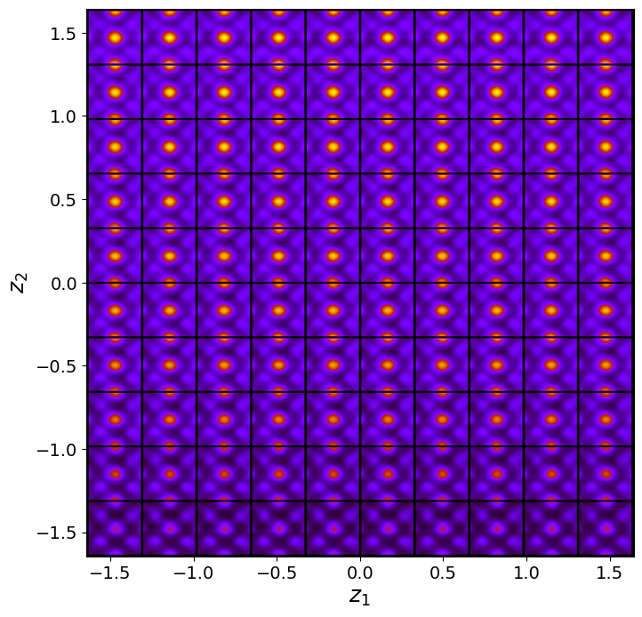
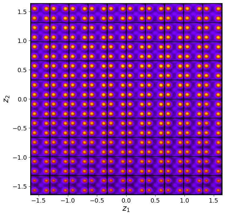
Ctvae_z_mean, Ctvae_z_sd = Ctvae.encode(train_data.unsqueeze(-1), lab_train)
print('no. of defects', Ctvae_z_mean.shape)

z1 = Ctvae_z_mean[:, -2]
z2 = Ctvae_z_mean[:, -1]
tx = Ctvae_z_mean[:, -4]
ty = Ctvae_z_mean[:, -3]
no. of defects torch.Size([10917, 4])
Latent representation
# fig_CtVAE_widget_1

# Define the data combinations you want to plot in the 4x3 grid
combinations = [
    (z1, z2, "z1", "z2"),
    (z1, tx, "z1", "tx"),
    (z1, ty, "z1", "ty"),
    (z2, tx, "z2", "tx"),
    (z2, ty, "z2", "ty"),
    (tx, ty, "tx", "ty"),
]

# Set up the figure with 3 rows and 3 columns (2 manifolds + 6 plots from combinations)
fig, axes = plt.subplots(3, 3, figsize=(18, 18))
axes = axes.flatten()

# (a) Manifold for condition 0
condition_0 = torch.nn.functional.one_hot(torch.tensor([0]), num_classes=2).float()
manifold_0 = generate_latent_manifold_C(n=10, decoder=Cvae.decode, target_size=(28, 28), condition=condition_0)
axes[0].imshow(manifold_0, cmap="gnuplot2", origin="upper", aspect="auto")
axes[0].set_xlabel("z1", fontsize=20, fontweight = "bold")
axes[0].set_ylabel("z2", fontsize=20, fontweight = "bold")
axes[0].set_xticks([])
axes[0].set_yticks([])
axes[0].text(-0.05, 1, 'a)', transform=axes[0].transAxes, fontsize=16, fontweight='bold', va='top', ha='right')

# (b) Manifold for condition 1
condition_1 = torch.nn.functional.one_hot(torch.tensor([1]), num_classes=2).float()
manifold_1 = generate_latent_manifold_C(n=10, decoder=Cvae.decode, target_size=(28, 28), condition=condition_1)
axes[1].imshow(manifold_1, cmap="gnuplot2", origin="upper", aspect="auto")
axes[1].set_xlabel("z1", fontsize=20, fontweight = "bold")
axes[1].set_ylabel("z2", fontsize=20, fontweight = "bold")
axes[1].set_xticks([])
axes[1].set_yticks([])
axes[1].text(-0.05, 1, 'b)', transform=axes[1].transAxes, fontsize=16, fontweight='bold', va='top', ha='right')

# Loop through combinations and plot KDE + scatter plots
for i, (x, y, xlabel, ylabel) in enumerate(combinations):
    ax = axes[i + 2]  # Start plotting from the 3rd subplot

    # Plot KDE with sns
    sns.kdeplot(x=x, y=y, ax=ax, cmap='Oranges', fill=True, alpha=0.4, levels=10)

    # Overlay scatter plot
    sns.scatterplot(x=x, y=y, ax=ax, hue=labels_c, palette='coolwarm', s=20, edgecolor="k", alpha=0.7, legend=False)

    # Set labels and axis properties
    ax.set_xlabel(xlabel, fontsize=20, fontweight = "bold")
    ax.set_ylabel(ylabel, fontsize=20, fontweight = "bold")
    ax.set_xticks([])
    ax.set_yticks([])
    ax.text(-0.05, 1, f'{chr(99 + i)})', transform=ax.transAxes, fontsize=20, fontweight='bold', va='top', ha='right')

# Hide unused subplot (if any extra subplots are created)
if len(combinations) + 2 < len(axes):
    for j in range(len(combinations) + 2, len(axes)):
        axes[j].set_visible(False)

# Adjust layout for better spacing
plt.tight_layout()

# Show the plot
plt.show()
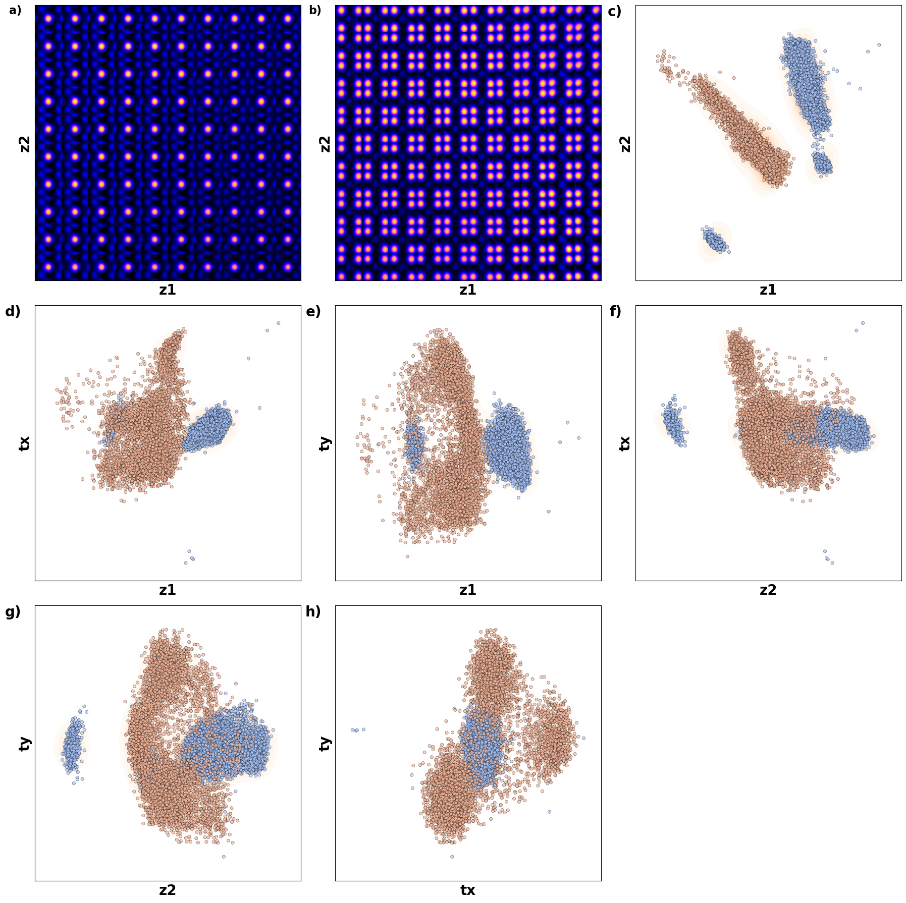
Latent maps
# fig_CtVAE_widget_2

# Define the data to plot
data = [
    (z1, "z1"),
    (z2, "z2"),
    (tx, "tx"),
    (ty, "ty"),
    (SBFOdata[1]["ab_Px_resized"][main[0]:main[1], main[2]:main[3]], "Ground Truth Px"),
    (SBFOdata[1]["ab_Py_resized"][main[0]:main[1], main[2]:main[3]], "Ground Truth Py")
]

# Set up the figure with 2 rows and 3 columns
fig, axes = plt.subplots(2, 3, figsize=(16, 10))
axes = axes.flatten()  # Flatten the array for easier indexing

# Loop through data and plot
for i, (values, title) in enumerate(data):
    if i < 4:  # For scatter plots
        scatter = axes[i].scatter(coms_target[:, 1], coms_target[:, 0], c=values, s=10, cmap='jet', marker="s")
    else:  # For imshow plots
        im = axes[i].imshow(values, cmap='jet', origin='lower')

    # Add titles and turn off axes
    axes[i].set_title(title, fontsize=16, fontweight="bold")
    axes[i].axis("off")

# Hide unused last subplot
if len(data) < len(axes):
    axes[-1].set_visible(False)

# Adjust layout for better spacing
plt.tight_layout()

# Show the plot
plt.show()
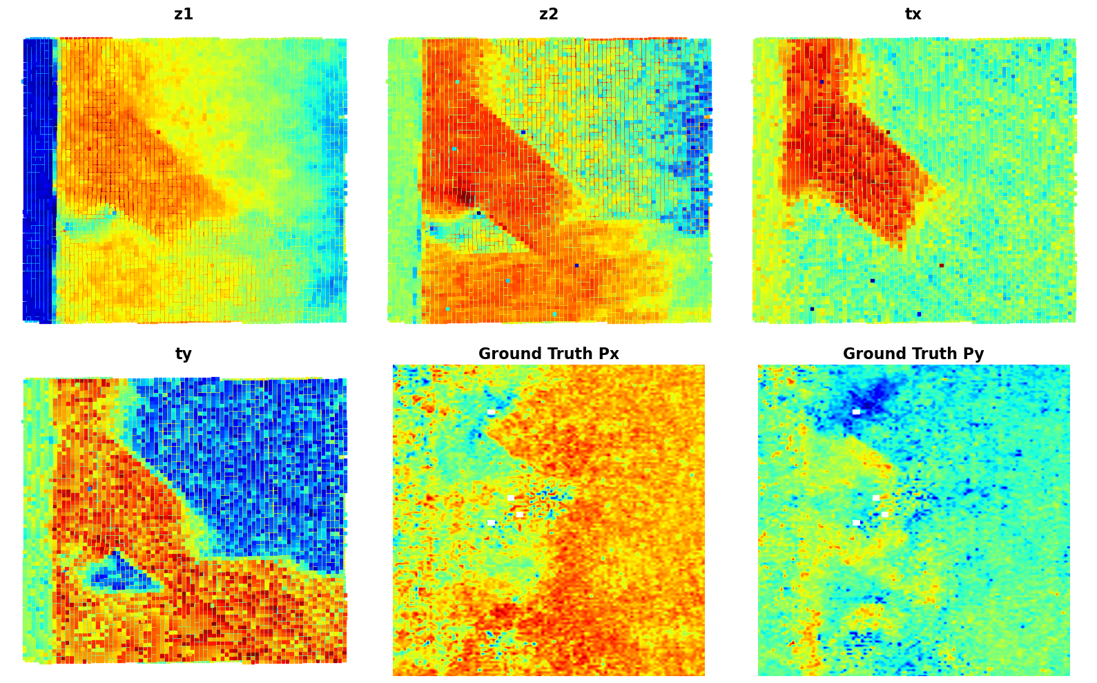
# Define the data to plot and corresponding titles, including ground truth Px and Py
data = [
    (z1, "z1"),
    (z2, "z2"),
    (tx, "tx"),
    (ty, "ty"),
    (SBFOdata[0]["ab_Px_resized"][main[0]:main[1], main[2]:main[3]], "Ground Truth Px"),
    (SBFOdata[0]["ab_Py_resized"][main[0]:main[1], main[2]:main[3]], "Ground Truth Py")
]

# Set up the figure with 2 rows and 3 columns (since we have 6 datasets to plot)
fig, axes = plt.subplots(2, 3, figsize=(15, 10))

# Flatten the axes array for easier looping
axes = axes.flatten()

# Loop through data and plot each in the respective subplot
for i, (values, title) in enumerate(data):
    if i < 4:  # Plotting z1, z2, tx, ty using scatter
        scatter = axes[i].scatter(coms_target[:, 1], coms_target[:, 0], c=values, s=10, cmap='jet', marker="s")
    else:  # Plotting Ground Truth Px and Py using imshow
        im = axes[i].imshow(values, cmap='jet', origin='lower')

    # Set title and turn off axis
    axes[i].set_title(title, fontsize=20, fontweight="bold")
    axes[i].axis("off")

    # Add subplot labels (a, b, c, etc.)
    axes[i].text(-0.05, 1, f'{chr(97 + i)})', transform=axes[i].transAxes,
                 fontsize=18, fontweight='bold', va='top', ha='right')

# Adjust layout for better spacing
plt.tight_layout()

# Show the plot
plt.show()
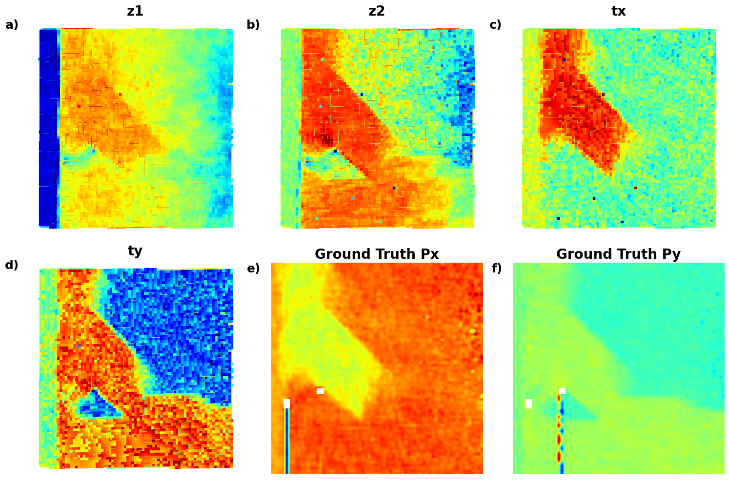
Here, looks like both z1,z2 and tx,ty contain information about domain strucutres. However, do we have too many latent variables here?
CtrVAE
in_dim = (window_size[0],window_size[1])

# Initialize vanilla VAE
Ctrvae = pv.models.iVAE(in_dim, latent_dim=2, c_dim = 2,  # Number of latent dimensions other than the invariancies
                     hidden_dim_e = [512, 512],
                     hidden_dim_d = [512, 512], # corresponds to the number of neurons in the hidden layers of the decoder
                     invariances=["r", "t"], seed=0)

# Initialize SVI trainer
trainer = pv.trainers.SVItrainer(Ctrvae)

# Train for n epochs:
for e in range(10):
    trainer.step(train_loader)
    trainer.print_statistics()

Ctrvae.save_weights('ctrvae_model')
print("Model saved successfully.")
Epoch: 1 Training loss: 769.7972
Epoch: 2 Training loss: 704.7175
Epoch: 3 Training loss: 690.6972
Epoch: 4 Training loss: 687.3008
Epoch: 5 Training loss: 685.3990
Epoch: 6 Training loss: 684.3206
Epoch: 7 Training loss: 683.6770
Epoch: 8 Training loss: 683.5209
Epoch: 9 Training loss: 682.8626
Epoch: 10 Training loss: 682.3796
Varitional Auto Encoder manifold representation
for cls in range(2):
    cls = pv.utils.to_onehot(tt([cls,]), 2)
    Ctrvae.manifold2d(d=10, y=cls, cmap="gnuplot")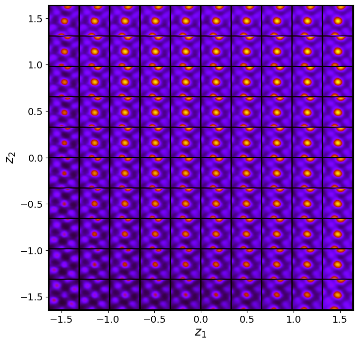
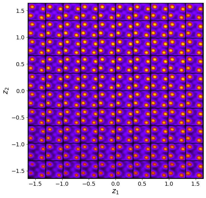
Ctrvae_z_mean, Ctrvae_z_sd = Ctrvae.encode(train_data.unsqueeze(-1), lab_train)
print('no. of defects', Ctrvae_z_mean.shape)

z1 = Ctrvae_z_mean[:, -2]
z2 = Ctrvae_z_mean[:, -1]
ang = Ctrvae_z_mean[:, 0]
tx = Ctrvae_z_mean[:, -4]
ty = Ctrvae_z_mean[:, -3]
no. of defects torch.Size([10917, 5])
Latent Representations
def plot_CrVAE_with_combinations():
    # Define the data combinations manually for all unique pairs
    combinations = [
        (z1, z2, "z1", "z2"),
        (z1, ang, "z1", r"$\theta$"),
        (z1, tx, "z1", "tx"),
        (z1, ty, "z1", "ty"),
        (z2, ang, "z2", r"$\theta$"),
        (z2, tx, "z2", "tx"),
        (z2, ty, "z2", "ty"),
        (ang, tx, r"$\theta$", "tx"),
        (ang, ty, r"$\theta$", "ty"),
        (tx, ty, "tx", "ty")
    ]

    # Set up the figure with 4 rows and 3 columns
    fig, axes = plt.subplots(4, 3, figsize=(18, 18))
    axes = axes.flatten()

    # Add the two manifolds as the first two plots
    condition_0 = torch.nn.functional.one_hot(torch.tensor([0]), num_classes=2).float()
    manifold_0 = generate_latent_manifold_C(n=10, decoder=Cvae.decode, target_size=(28, 28), condition=condition_0)
    axes[0].imshow(manifold_0, cmap="gnuplot2", origin="upper", aspect="auto")
    axes[0].set_xlabel(r"$z_1$", fontsize=20, fontweight="bold")
    axes[0].set_ylabel(r"$z_2$", fontsize=20, fontweight="bold")
    axes[0].set_xticks([]), axes[0].set_yticks([])
    axes[0].text(-0.1, 1.05, '◊ a)', transform=axes[0].transAxes, fontsize=20, fontweight='bold', va='top', ha='right')

    condition_1 = torch.nn.functional.one_hot(torch.tensor([1]), num_classes=2).float()
    manifold_1 = generate_latent_manifold_C(n=10, decoder=Cvae.decode, target_size=(28, 28), condition=condition_1)
    axes[1].imshow(manifold_1, cmap="gnuplot2", origin="upper", aspect="auto")
    axes[1].set_xlabel(r"$z_1$", fontsize=20, fontweight="bold")
    axes[1].set_ylabel(r"$z_2$", fontsize=20, fontweight="bold")
    axes[1].set_xticks([]), axes[1].set_yticks([])
    axes[1].text(-0.1, 1.05, '◊ b)', transform=axes[1].transAxes, fontsize=20, fontweight='bold', va='top', ha='right')

    # Loop through combinations and plot KDE with scatter plots
    for i, (x, y, xlabel, ylabel) in enumerate(combinations):
        ax = axes[i + 2]  # Start from the third subplot

        # Plot KDE first
        sns.kdeplot(x=x, y=y, ax=ax, cmap='Oranges', fill=True, alpha=0.4, levels=10)

        # Overlay scatter plot
        sns.scatterplot(x=x, y=y, ax=ax, hue=labels_c, palette='coolwarm', s=20, edgecolor="k", alpha=0.7, legend=False)

        # Set labels and axis properties
        ax.set_xlabel(xlabel, fontsize=20, fontweight='bold')
        ax.set_ylabel(ylabel, fontsize=20, fontweight='bold')
        ax.set_xticks([])
        ax.set_yticks([])
        ax.text(-0.1, 1.05, f'◊ {chr(99 + i)})', transform=ax.transAxes, fontsize=20, fontweight='bold', va='top', ha='right')

    # Hide unused subplots to avoid empty maps
    for j in range(len(combinations) + 2, len(axes)):
        axes[j].set_visible(False)

    # Adjust layout for better spacing
    plt.tight_layout()

    # Show the plot
    plt.show()
# fig_CtrVAE_widget_1

plot_CrVAE_with_combinations()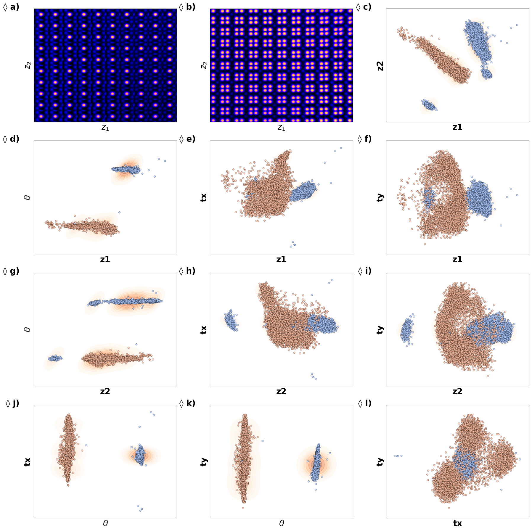
# # Define the data combinations manually for all unique pairs
# combinations = [
#     (z1, z2, "z1", "z2"),
#     (z1, ang, "z1", "ang"),
#     (z1, tx, "z1", "tx"),
#     (z1, ty, "z1", "ty"),
#     (z2, ang, "z2", "ang"),
#     (z2, tx, "z2", "tx"),
#     (z2, ty, "z2", "ty"),
#     (ang, tx, "ang", "tx"),
#     (ang, ty, "ang", "ty"),
#     (tx, ty, "tx", "ty")
# ]

# # Set up the figure with 4 rows and 3 columns (enough to hold all combinations)
# fig, axes = plt.subplots(4, 3, figsize=(16, 16))

# # Flatten the axes array to loop through easily
# axes = axes.flatten()

# # Loop through combinations and plot them
# for i, (x, y, xlabel, ylabel) in enumerate(combinations):
#     # Plot KDE first
#     sns.kdeplot(x=x, y=y, ax=axes[i], cmap='Spectral', fill=True, alpha=0.4, levels=10)

#     # Scatter plot on top of KDE
#     scatter = axes[i].scatter(x, y, c=labels_c, s=20, alpha=0.7, edgecolors="k", cmap='jet')

#     # Set labels and axis properties
#     axes[i].set_xlabel(xlabel, fontsize=18)
#     axes[i].set_ylabel(ylabel, fontsize=18)
#     axes[i].set_xticks([])
#     axes[i].set_yticks([])

# # Hide unused subplots to avoid empty maps
# for j in range(len(combinations), len(axes)):
#     axes[j].set_visible(False)

# # Adjust layout for better spacing
# plt.tight_layout()

# # Show the plot
# plt.show()
Latent maps
# fig_CtrVAE_widget_2

# Define the data to plot and corresponding titles, including ground truth Px and Py
data = [
    (z1, "z1"),
    (z2, "z2"),
    (tx, "tx"),
    (ty, "ty"),
    (ang, "ang"),
    (SBFOdata[0]["ab_Px_resized"][main[0]:main[1], main[2]:main[3]], "Ground Truth Px"),
    (SBFOdata[0]["ab_Py_resized"][main[0]:main[1], main[2]:main[3]], "Ground Truth Py")
]


# Set up the figure with 3 rows and 3 columns (since we have 7 datasets to plot)
fig, axes = plt.subplots(3, 3, figsize=(18, 18))

# Flatten the axes array for easier looping
axes = axes.flatten()

# Loop through data, plot each in the respective subplot
for i, (values, title) in enumerate(data):
    if i < 5:  # Plotting latent variables and physical variables
        scatter = axes[i].scatter(
            coms_target[:, 1], coms_target[:, 0], c=values, s=10, cmap='jet', marker="s"
        )
        # axes[i].set_xlim(x_min, x_max)
        # axes[i].set_ylim(y_min, y_max)
    else:  # Plotting Ground Truth Px and Py
        im = axes[i].imshow(values, cmap='jet', origin='lower')

    axes[i].set_title(title, fontsize=20, fontweight="bold")
    axes[i].text(-0.05, 1, f'{chr(97 + i)})', transform=axes[i].transAxes, fontsize=20, fontweight='bold', va='top', ha='right')
    axes[i].axis("off")

# Hide the unused subplot to avoid empty maps
for j in range(len(data), len(axes)):
    axes[j].set_visible(False)

# Adjust layout for better spacing
plt.tight_layout()

# Show the plot
plt.show()
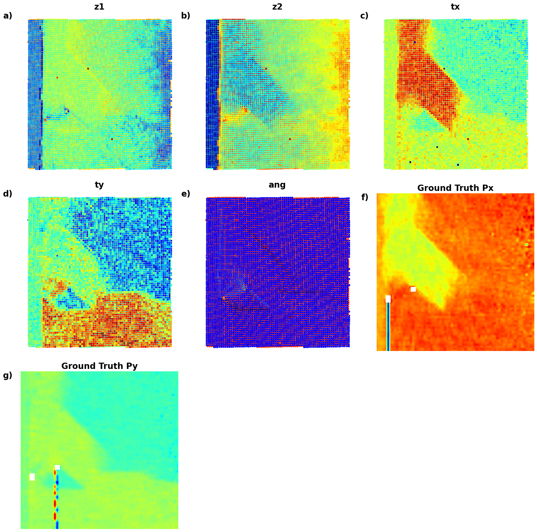
# Define the data to plot and corresponding titles, including ground truth Px and Py
data = [
    (z1, "z1"),
    (z2, "z2"),
    (tx, "tx"),
    (ty, "ty"),
    (ang, "ang"),
    (SBFOdata[1]["ab_Px_resized"][main[0]:main[1], main[2]:main[3]], "Ground Truth Px"),
    (SBFOdata[1]["ab_Py_resized"][main[0]:main[1], main[2]:main[3]], "Ground Truth Py")
]

# Set up the figure with 3 rows and 3 columns (since we have 7 datasets to plot)
fig, axes = plt.subplots(3, 3, figsize=(15, 12))

# Flatten the axes array for easier looping
axes = axes.flatten()

# Loop through data, plot each in the respective subplot
for i, (values, title) in enumerate(data):
    if i < 5:  # Plotting latent variables and physical variables
        scatter = axes[i].scatter(coms_target[:, 1], coms_target[:, 0], c=values, s=10, cmap='jet', marker="s")
    else:  # Plotting Ground Truth Px and Py
        im = axes[i].imshow(values, cmap='jet', origin='lower')

    axes[i].set_title(title, fontsize=20)
    axes[i].axis("off")

# Hide the unused subplot to avoid empty maps
for j in range(len(data), len(axes)):
    axes[j].set_visible(False)

# Adjust layout for better spacing
plt.tight_layout()

# Show the plot
plt.show()
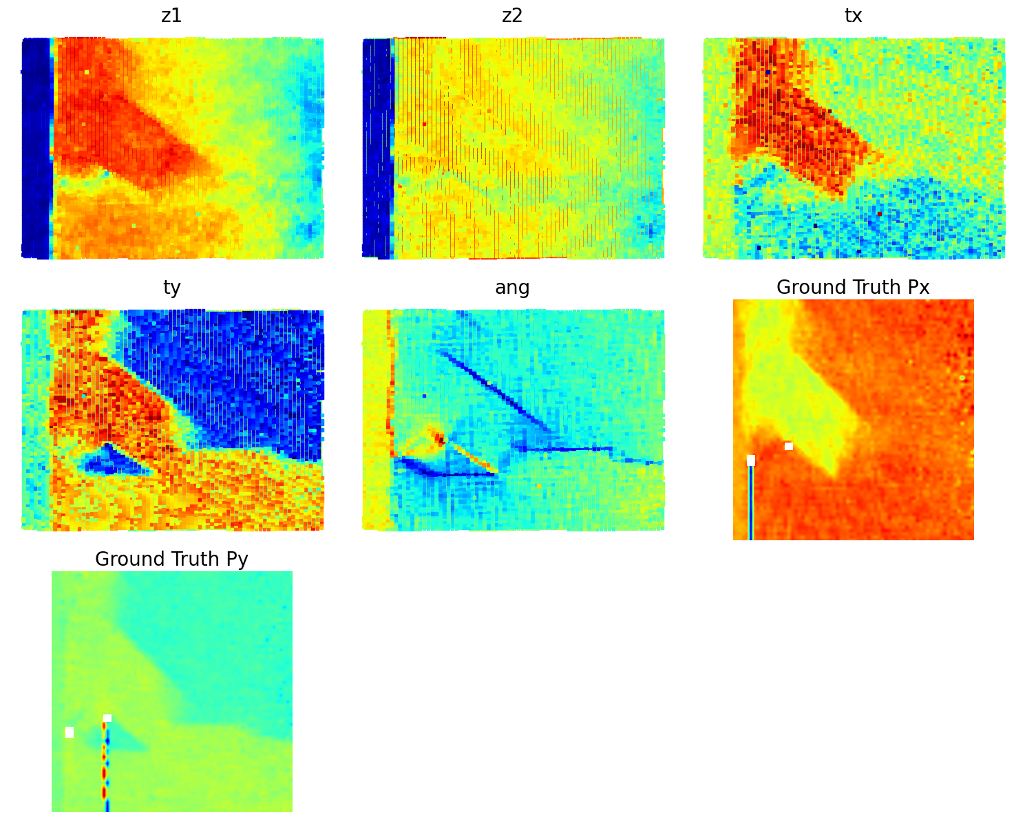
Now, it looks like we definitely have too many latent variables - our information starts to become somewhat redundant. Compare the z2 and angle.
Sumamry: Troughout htis notebook, we have taken you on the whirlwind tour of the invariant and conditional VAEs. By intorducing the invariances, we both allow the data to speak for itself (via latent variables), and separate physical meaning (translations and rotations). We have also tried to explain the logic that we can follow in choosing the right VAE, going forward and backward between the data and physical interpetations and expectations. ALready in this form, you can use thi snotebook for your own data sets - whether these are ferroics, multiphase materials, or otehr systems.
However, you can also ask questions:
- How do we know that the number of latents and chosen invariances are correct?
- How do we know which descriptor to choose (here we use the patch of size w, and w can be a variable. Also, we can choos emore complex descriptors, e.g. rectangular pathcches w1,w2, or even more complex objects)
- What about more complex invariances?
After all, here we eseentially did iterative epxloration in small, but still combinatorial space. It turns out, we can optimize thes eparameters using the reward function based approach - stand by for futher papers form our group!

