We begin our survey on transfer learning protocols by looking at the primary high-level constraints and decisions made in the transfer learning workflow: the amount of data available in the transfer domain, whether or not the whole model is re-trained, and optimization hyperparameters. In data scarce settings, perhaps the most important factor in transfer learning is the amount of high-quality data one has available in the transfer learning domain to use for training. We explore the dependence of model performance (best validation performance) in the transfer domain on the transfer dataset size in Figure 6.1 (left). During transfer learning, our trained models have access to datasets one-eighth the size (64 examples, the equivalent one 4k by 4k acquisition), one-fourth the size (128 examples), half the size (256 examples), or, in the extreme case, of equal size (512 examples) to their original training dataset. As could be expected, models trained with more data in their target domain tend achieve a lower loss and thus perform better. While all of these model distributions have high performing models, model performance variance also decreases with increased dataset size, indicating that having more data makes it also more likely to train a successful model. We can see, also, the overall proportion of the worst performing models (i.e., the right-hand tail of the model distribution) grows quickly as models are trained on fewer new images, indicating that using especially small transfer learning datasets can significantly increase the likelihood of a model having unacceptably poor performance, which can be difficult to overcome without the opportunity to train a large number of models.

Source:Effect of training hyperparameters

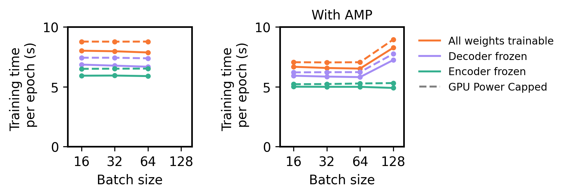
Another common step taken during transfer learning is to freeze a portion of the weights of a model, which prevents the weights from being updated and further optimized during the second phase of training. While unambiguously interpreting the functions of subsets of neural network models is difficult, weight freezing can greatly reduce the training cost, time, and energy consumption of model training and provides a discrete way to specifically tune parts of a machine learning model. Here, we experiment with three weight-freezing procedures: the first, in which we freeze the ‘encoder’ portion of the U-Net (the downsampling residual blocks); the second, in which we freeze the ‘decoder’ half of the U-Net (the upsampling blocks); and the third, in which we leave all weights optimizable. Often, a default choice of transfer learning is to freeze the ‘feature’ part of the neural network, which, under such an interpretation, would semantically correspond to freezing the encoder portion of the U-Net. As shown in Figure 6.1 (middle), freezing the decoder weights can provide comparable performance to fine-tuning the whole model, while freezing the encoder weights slightly degrades transfer learning performance. Importantly, in our case study, freezing the encoder weights reduces the number of trainable parameters by almost 80%, which reduce the training time by about 15-25% and mildly reduces training memory consumption (c.f. Figure 6.2). For larger or more complex models, combining selective weight freezing alongside other training techniques such as automated mixed precision training could provide substantial improvements in training time and model scalability.

The effect of other optimization-related hyperparameters, such as the learning rate (i.e., gradient step size) of the optimizer, are a bit more straightforward to understand. Within a fixed training budget, such as our experiment with only 10 training epochs per stage, changes in learning rate can decently impact performance (c.f. Figure 6.1, right). For our models, using the most aggressive learning rates in both phases lead to both the best model performance and the smallest variance of model performance. We note, though, that without constraints on training budgets, empirical results suggest that similar levels of performance can be achieved regardless of the convergence rate as long as convergence occurs stably Shallue et al., 2018Godbole et al., 2023.